Calibrating the Network Analyzer

The network analyzer must be calibrated before any S-parameter measurements are performed. The system must be allowed to warm up for at least 1 hour before calibration, and the calibration standards must be at ambient room temperature. It is a good practice to switch on the analyzer and expose the calibration devices to air before you make the DC measurements.

Good calibration of the network analyzer system is critical to a good high-frequency measurement and extraction. A good calibration is dependent on the quality of the calibration kit standard devices, the care with which they are maintained, and the correctness and repeatability of the device connections. A stable ambient temperature (±1°C) is required to maintain a good calibration.

For the high-frequency IC-CAP measurement procedures, the network analyzer is calibrated over a broadband frequency range, to perform the S-parameter measurements for AC and parasitic extractions. In addition, one or two calibrations may be needed at CW frequencies for specific measurement setups. These procedures explain how to set up a broadband calibration and a separate CW calibration. For the Agilent 8753 and 8720 systems, IC-CAP does not support the subset calibration technique used for an Agilent 8510 system.

The instructions given here are very abbreviated: more detailed information is available in the Agilent 8753 operating manual.

To connect the network analyzer:

Disconnect the terminations from the bias networks. Connect the RF cables from the network analyzer test ports to the RF inputs of the bias networks.

Swept Broadband Calibration

1	In the IC-CAP model, select the S-parameter setup of your choice.

2	In the measurement setup, set the instrument options appropriately for your measurement. (See Defining the Instrument States for S-Parameter Measurements.)

3	You can set the network analyzer manually from its front panel, or use the IC-CAP Calibrate command in the setup menu to download the instrument options into the network analyzer. In either case, you perform the cal standards measurements at the analyzer front panel.

4	The following steps explain how to perform a manual network analyzer front panel calibration.

5	On the network analyzer, press LOCAL to gain front panel control. Press PRESET to return to a known standard state.

6	If you are using a system with the 6 GHz receiver option and you wish to measure in the 3 MHz to 6 GHz range, press SYSTEM > FREQ RANGE 3GHz6GHz.

7

To define the frequency range of the calibration and measurement, press START, and use the numerical keypad to set the start frequency, ending with one of the terminator keys (such as G/n) at the right of the keypad. Similarly, press STOP and set the stop frequency. Set a frequency range at least as wide as the operating range of the device.

8	Press MENU > NUMBER OF POINTS, and enter the number of points to be measured across the range. Allow enough points to provide good measurement resolution: at least 51 points are recommended.

9	Press MENU > TRIGGER MENU > CONTINUOUS to set a continuous stimulus sweep.

10

Press MENU > POWER, and set the desired power level. In setting the source power and test set attenuation, take care that the power level will not be excessive at the device input. Also consider the gain of the device, and set a power level that will not saturate the input port samplers of the analyzer. If a receiver input is overloaded (>+14 dBm), the analyzer automatically reduces the output power of the source to -85 dBm and displays the error message OVERLOAD ON INPUT (R, A, B) POWER REDUCED. In addition, the annotation P appears in the left margin of the display to indicate that the power trip function has been activated. When this occurs, reset the power to a lower level, then toggle the SOURCE PWR on/OFF softkey to switch on the power again.

11	For a device with power dropoff at higher frequencies, you may wish to set a power slope using the SLOPE ON/off softkey. An appropriate power slope would be in the region of 2-3 dB/GHz.

12

Press AVG > AVERAGING FACTOR, and enter an averaging factor high enough to reduce trace noise and increase dynamic range as appropriate for your device measurements. A good default averaging factor is 256. To speed your measurements, you may find it convenient to set an averaging factor as low as 16. Press AVERAGING ON.

13

You can further reduce the noise floor by reducing the receiver input bandwidth. Press IF BW, and enter one of the following allowed values in Hz: 3000, 1000, 300, 100, 30, or 10. A tenfold reduction in IF bandwidth lowers the measurement noise floor by about 10 dB; however, the sweep time may be slower. For more information on averaging and the different trace noise reduction techniques, refer to the Agilent 8753 operating manual.

14	Press CAL > CAL KIT, and select the appropriate default or user-defined cal kit for your calibration devices.

15	If you wish to modify an internal calibration kit definition (see below), do so now.

16

Press CAL > CALIBRATE MENU, and perform the calibration of your choice at the analyzer front panel, measuring each of the standard devices in turn and pressing the softkeys as each measurement is complete. A full two-port cal provides the greatest accuracy. A TRL* or LRM* cal is an appropriate alternative for in-fixture measurements. Omit isolation cal. Press DONE, and save the cal in the register number specified in the instrument options table. This must be a different register than you use for any CW cal.

17	Detailed procedures for measurements of calibration standards are provided in the Agilent 8753 operating manual.

CW Frequency Calibration

1	To set the CW frequency, press MENU > CW on the analyzer, and enter the frequency using the numerical keypad and one of the terminator keys.

2	Make a separate set of standards measurements.

3	When you save the calibration, use the cal register number specified in the instrument options table for this CW cal. This must be a different register than you used for the swept cal or any other CW cal.

After the network analyzer is calibrated, return to the modeling chapter you are using for the S-parameter measurement procedures.

Using the Automatic IC-CAP Calibrate Function

Alternatively, you can use the IC-CAP Calibrate command for a broadband or CW calibration. This downloads the instrument states from IC-CAP to the network analyzer before you perform a calibration with the analyzer. This helps to avoid errors in matching values set in the analyzer and in IC-CAP.

1	In the IC-CAP model, select the S-parameter setup of your choice.

2	In the measurement setup, set the instrument options appropriately for your measurement.

3	From the setup menu select Calibrate. The instrument options are downloaded into the analyzer, together with the frequency stimulus values set in the Inputs.

4	The message Calibrate HP8753.7.16 before measuring is displayed. Select OK and perform the cal standards measurements from the analyzer front panel. Save the cal in the register specified in the instrument options.

Modifying a Cal Kit Definition

The network analyzer's internal calibration kit models are accurate for use with the standard coaxial calibration kits defined for use with the Agilent 8753. In certain circumstances, however, you may need a user-defined kit for compatibility with your calibration standards. Some possible cases might be these:

•	The impedance of an on-wafer load may not be exactly 50. You can characterize the DC impedance of a load exactly with a precision ohmmeter measurement, and enter the impedance value into the cal kit definition.

The procedure to modify an internal cal kit definition is complex, and not to be undertaken without a solid understanding of error correction and the system error model. It is explained in detail in Product Note 8510-5, Specifying Calibration Standards for the Agilent 8510 Network Analyzer (Agilent literature number 5954-1559). For information specific to the Agilent 8753 network analyzer, including an example procedure, refer to the Agilent 8753 operating manual.

For information on the characteristics of calibration standards used with a fixture or probe station, refer to the manufacturer's device data sheets or other documentation.

TRL* Calibration Under IC-CAP Control

The Agilent 8753D network analyzer has the capability to perform a TRL* or LRM* calibration using internal firmware. TRL* (TRL-star) is an implementation of TRL that has been adapted for three-sampler network analyzers for use in fixtured measurement environments. (Note that this requires that you modify a user cal kit definition: see above.)

Earlier models of the Agilent 8753 do not have the internal TRL* calibration capability. The IC-CAP procedure described in the following pages allows you to perform a similar Agilent 8753C calibration using TRL cal standards compatible with your fixture. IC-CAP calculates the error coefficients and downloads them into the network analyzer. The procedure can be used for either a TRL* (thru-reflect-line) or TRM* (thru-reflect-match) calibration.

When the calibration is complete, the reference plane is defined at the middle of the thru standard, or at the interface to the DUT when it is installed in the compatible carrier.

For more information about TRL* calibration, refer to Product Note 8720-2, In-fixture microstrip device measurements using TRL* calibration, Agilent literature number 5091-1943E.

The IC-CAP software for the TRL* calibration is in the model file TRLCAL.mdl. Find the TRL* calibration model under:

/examples/model_files/misc/TRLCAL.mdl

The message WARNING: HP8753.7.16 Options saved in TRLCAL/cal/short (or another filename) may be displayed. In this case, you will need to perform a Rebuild, as explained under Performing Hardware Setup in IC-CAP.

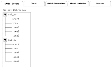
The TRL* Calibration DUTs and Setups

The following figure illustrates the DUTs and setups for TRLCAL.mdl.

The SETUPs are used to collect the measured raw S-parameters of various TRL (or TRM) standards, using variable values defined by you in the macros. IC-CAP computes the required error coefficients from this raw S-parameter data.

Figure 206 TRLCAL DUT/Setup Panel

The TRL* calibration uses separate setups for a swept frequency cal (cal_sw) and a CW frequency cal (cal_cw), which are both required in some modeling procedures. For the Agilent 8753 and 8720 systems, IC-CAP does not support the subset calibration technique used for an Agilent 8510 system, therefore two sets of standards measurements are required. IC-CAP stores measured data in the setups for both the swept and CW cals.

The README macro provides an abbreviated set of instructions for the TRL* calibration procedure. The other macros provide interactive prompts for defining the instrument states and calibration frequencies, and for performing the calibration.

Definitions: Standards and Measurement Setups

The IC-CAP TRL* calibration requires measurements of three or more standard devices: a short, a thru, and at least one line standard (for TRL*) or match standard (for TRM*). The performance characteristics of the standards must be specified over the frequency range of the calibration. Therefore it may be necessary to use as many as three line standards to cover the total frequency range for a swept frequency cal. If so, you will need to define the transition frequencies between the line standards.

Measurement Setups

The setups in the TRLCAL model measure the calibration standards, and store the measured raw S-parameter data in files with the same names as the setups. Each standard is measured over the full frequency range of the calibration. However, if multiple line standards are used, IC-CAP processes only the data delimited by the transition frequencies to compute the error coefficients of each. For a CW cal, IC-CAP processes only the data measured at the CW frequency you specify. The setups are used as follows:

Short:

Measures the short standard and stores the measured data.

Thru:

Measures the thru standard and stores the measured data.

LineA:

Measures the first (lowest frequency) line standard and stores the measured data. In calculating the error coefficients for a swept frequency cal, IC-CAP uses only the data from the start frequency to the first transition frequency, or to the stop frequency if an above-range or zero-value first transition is defined. (You will define the calibration range and the transition frequencies later in the procedure.) The lineA standard can be represented either by a length of transmission line for a TRL* cal, or by a matched load for a TRM* cal.

LineB:

Measures the second line standard (if any) and stores the measured data. In calculating the error coefficients for a swept frequency cal, IC-CAP uses only the data from the first transition frequency to the second transition frequency, or to the stop frequency if an above-range or zero-value second transition is defined. Typically the standard measured is a length of transmission line different from either the thru or lineA standards.

LineC:

Measures the third line standard (if any) and stores the measured data. In calculating the error coefficients for a swept frequency cal, IC-CAP uses only the data from the second transition frequency to the stop frequency. Typically the standard measured is a length of transmission line different from either the thru, lineA, or lineB standards.

Transition Frequencies of Line Standards

Your calibration kit may have only one line (or match) standard, or it may have more than one line standard, each specified over a portion of the total specified cal kit frequency range. Refer to the data sheet for your calibration kit to determine the specified frequency ranges of each of the devices. For the RF frequency range you wish to measure, you may need to measure all the line standards, or you may need to measure only one or two. If you measure more than one line standard, the specified upper frequency limit for the first line standard is the first transition frequency. Similarly, the specified upper frequency limit for the second line standard is the second transition frequency.

For example, if your total measurement frequency range is 300 kHz to 6 GHz and your first line standard is specified from 300 kHz to 1 GHz, then your first transition frequency is 1 GHz. If your second line standard is specified from 1 GHz to 5 GHz, then your second transition frequency is 5 GHz.

The TRLCAL.mdl file provides for measurements of up to three line standards for a swept frequency cal. If you use only one or two, you can define transition frequencies above the range of the calibration, and IC-CAP defaults to the start and/or stop frequencies. For example, if your total measurement frequency range is 300 kHz to 3 GHz and your second line standard is specified from 1 GHz to 5 GHz, you can set the second transition frequency to 5 GHz (or 0), and IC-CAP will measure the second line from 1 GHz to 3 GHz.

Measurement Setup Names vs. Actual Standards Names

The measurement setup names may not correspond with the names of the standards in your calibration kit. It is important to understand that the setup names are only filenames for the measured data. The actual fixtured standards you use for the line measurements will depend on the frequency range of your calibration, not on the names of the setups.

You must use the lineA setup for your lowest frequency line (or match) measurement, even if the cal standard you use is not line 1 in your calibration kit. This is because IC-CAP processes measured data from the setup files in the sequence they are shown in the model editor window. If a file is left empty (for example lineA), IC-CAP will stop processing data, even if there is measured data in lineB or lineC.

For example, you may have a calibration kit with a frequency range of 300 kHz to 6 GHz, and you may be calibrating for device measurements over a range of only 5 GHz to 6 GHz, using a short, a thru, and a single line (or match) standard. In this case, you will use the lineA setup to measure your line or match standard that is specified for performance over the 5 GHz to 6 GHz frequency range, no matter how it is labeled.

If you are performing a CW cal alone, you must use the lineA setup for your line or match measurement.

Defining the IC-CAP TRL* Cal Instrument States

IC-CAP controls the network analyzer in measuring the calibration standards. These procedures configure IC-CAP with the required network analyzer instrument states to measure the TRL* calibration standards for the swept frequency and CW frequency cals for both the Agilent 8753D and earlier-model Agilent 8753s. (Instrument states are similar for Agilent 8720-family instruments, and are explained in Chapter 1, "Supported Instruments," in the IC-CAP Reference manual.) The Instr_opts macro lets you define the instrument state once for each cal and load it into all the corresponding measurement setups.

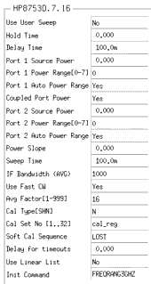
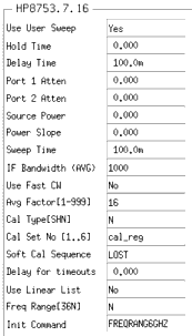
1	Select the Macros tab. Select the Instr_opts macro, and Execute. The instrument options window illustrated in the following figure is for the short setup for a swept frequency cal using an Agilent 8753D.

Figure 207 TRL* Cal Instrument States for Swept Measurements with Agilent 8753D

2

In the dialog box, select OK as prompted, then make any instrument state changes required for your calibration and measurements, using the illustrations and the following instructions for guidance. The illustrated values are typical defaults for a TRL* calibration used for measuring BJTs. The settings you use may be different, depending on the characteristics of the devices you intend to measure and model.

Swept Measurements with Agilent 8753D

1	For swept measurements, set Use User Sweep to No because this is a standard internal sweep.

2	Set the source power level in dBm to 0.000 for measurements below 3 GHz. For measurements above 3 GHz, 20.00 is appropriate. The power levels are tied to the frequency range set in Init Command, below.

3	1000 Hz is a good default value for IF bandwidth. Reducing the IF bandwidth lowers the noise floor, at the cost of slowing the sweep speed. Allowed IF bandwidth values in hertz are 3000, 1000, 300, 100, 30, and 10.

4	Set Use Fast CW to Yes for a swept frequency measurement, to minimize repeated switching between the test set ports.

5	Cal Type (SHN) refers to software/hardware/none. Set it to N for "none." This is because the measurements you will make in this cal procedure are uncalibrated measurements. The finished calibration set will be used in your later measurement and modeling procedures.

6	Set Cal Set No to cal_reg, a variable used by the program.

7	The setting you use for Soft Cal Sequence is irrelevant, since Cal Type is set to None.

8	Set Use Linear List to No, otherwise the Agilent 8753 will be set to frequency list mode.

9	Set Init Command to FREQRANG3GHZ if you are using a standard Agilent 8753 network analyzer. (If you are using an Agilent 8753 with the 6 GHz extended frequency option and measuring above 3 GHz, enter FREQRANG6GHZ.)

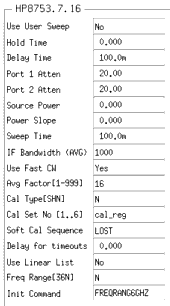
Swept Measurements with Earlier-Model Agilent 8753

The window illustrated in the following figure is for the short setup for a swept frequency cal using an earlier-model Agilent 8753.

Figure 208 TRL* Cal Instrument States for Swept Measurements with Earlier-Model Agilent 8753 (>3 GHz)

We recommend you use the same attenuator settings at port 1 and port 2, since the earlier Agilent 8753 analyzer uses the same attenuator for both ports. In setting power levels, you will need to set a source power sufficient to maintain phase lock, while taking care not to saturate the device output. Settings of 10 to 20 dB attenuation at both ports with a source power level of 0 dBm are appropriate for many devices with gain.

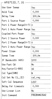
CW Measurements

1	Some of the instrument state settings for the TRL* CW cal are the same as for the swept frequency cal. The following settings are different, as illustrated:

Figure 209 TRL* Cal Instrument States for CW Measurements with Agilent 8753D

2	For CW measurements, set Use User Sweep to Yes.

3	You may not need to set attenuation for CW measurements, since gain may not be a factor. The CW measurements are usually used to determine the junction capacitance of a device. For this purpose the device is biased in such a way that it has loss rather than gain.

4	Set Use Fast CW to No.

Figure 210 TRL* Cal Instrument States for CW Measurements, Earlier Agilent 8753

5	When you have completed the settings, select the Instr_dupl macro, and Execute. This macro loads the short instrument options for the swept frequency cal into the other cal_sw setups; and the short options for the CW cal into the other cal_cw setups (thru, lineA, lineB, lineC).

6	A message in the UNIX window will tell you when the instrument options are duplicated in all the setups. Ignore any does not cascade warnings.

Defining the Calibration Frequencies

You define the values for frequency range, number of measurement points, and transition frequencies between line standards in the Cal_freqs macro, as follows:

1	Select the Cal_freqs macro, and Execute. A dialog box will be displayed.

2	Enter the start frequency for your swept frequency calibration as prompted, and select OK.

3	Enter the stop frequency and select OK. The stop frequency must be greater than the start frequency.

4	At the prompt to enter the number of frequency points, use one of the following Agilent 8753 allowable values:

3	11	26	51
101	201	401	801
1601

5	If you are doing a CW cal along with the swept cal, enter the CW frequency. If not, enter 0. (If you are doing a CW cal alone, refer to the Note below.) Select OK.

6	If you are using more than one line/match standard, enter the transition frequency for the first line (between lineA and lineB). Select OK.

7	If you are using three line standards, enter the transition frequency for the second line (between lineB and lineC). Select OK.

8	If you are using only one or two line standards, enter above-range or zero-value transition frequencies for the setups that do not apply. IC-CAP will measure only from the start to the stop frequency.

Refer to the paragraphs under Definitions: Standards and Measurement Setups for explanations of transition frequencies and the difference between the software setup names and the hardware standards names. The information there can prevent possible problems in the way IC-CAP processes the data.

9	When you have defined all the calibration frequencies, the UNIX window will list them, and will conclude with the message Completed.

Performing the Calibration

The Calibration macro provides a series of prompts to guide you through the standards measurements. In this part of the procedure, you follow the prompts to connect the defined standards, and instruct IC-CAP to measure them. You then specify network analyzer registers to store the swept and CW calibrations, and IC-CAP calculates the error coefficients from the measured raw S-parameter data, then downloads them into the analyzer registers.

1	Select the Calibration macro, and Execute.

2

IC-CAP displays a dialog box, prompting you to perform the standards measurements you have defined. In each case, first connect the standard, then respond to the prompt by entering s for short, t for thru, A for the lineA setup, B for the lineB setup, and C for the lineC setup. Each time you enter a single letter, press Return. A message in the UNIX window tells you the standard is measured.

3

Following this prompt sequence, a dialog box asks you Done? [y/n]. If all the necessary cal standards have been measured, type y and select OK. (If you want to remeasure a standard, type n, reconnect the device, and type the appropriate character for the device setup. IC-CAP will remeasure, and replace the old data with the new.)

4

The next dialog box asks you to enter the calibration storage register for the swept cal. Type in a number between 1 and 4, and select OK. (Do not use register 5, because IC-CAP reserves it for temporary storage.) IC-CAP calculates the error coefficients, downloads them into the network analyzer, and turns on the analyzer calibration.

5	Next enter a different register number for the CW calibration, and select OK. IC-CAP performs the CW cal and downloads it.

6	The instrument state and calibration are saved in the analyzer's short-term non-volatile memory (that is, even if the instrument is switched off for as long as 72 hours).

7	Whenever you use these swept and CW TRL* calibrations for a modeling procedure, enter the corresponding register numbers in the Cal Set No field of the IC-CAP instrument options window. Also set the Cal Type (SHN) field to H for hardware.

If you wish to verify the calibration, you can return the network analyzer to local operation and make a calibrated thru measurement.

Saving the Calibration Data in IC-CAP

When the calibration is complete, save the model file with the measured standards data in it, so that you can always quickly retrieve the error coefficients and re-enter them into the network analyzer:

1	Select File > Save As.

2

In the dialog box that appears, type in an appropriate pathname and filename. Examples of possible filenames might include the calibration date or frequency, such as TRLCAL_101597.mdl or TRLCAL_6GHz.mdl. Select OK. First the CW cal is saved in one analyzer register using the variable cal_reg_cw; then the swept cal is saved in another register using the variable cal_reg_sw.

3

When you want to retrieve the error coefficients at some future time, read in the .mdl file you saved. Select the thru setup for either the swept or CW cal. Make sure the Agilent 8753 instrument state corresponds exactly to the instrument options in the thru setup. Select the CalHP8753 transform, and Execute. IC-CAP will calculate the error coefficients, download them into the network analyzer, and turn on the analyzer calibration.

Press LOCAL on the analyzer to return it to front panel control, then press SAVE and a register softkey to save the cal in one of the analyzer's memory registers.

This ends the procedures for TRL* calibration under IC-CAP control.