Print version of this Book (PDF file)
Non-Parametric Analysis
IC-CAP Statistics contains an exclusive feature called Non-Parametric Boundary Analysis. Unlike other statistical analysis tools, which only handle Gaussian distributions, Non-Parametric Boundary analysis uses a new technique to handle arbitrary data distributions, Gaussian or non-Gaussian, and selects nominal and boundary models. Non-parametric analysis works for any data from any arbitrary stochastic process.
Because Non-Parametric Boundary Analysis is a new technique and not described in statistical textbooks, we will describe this method here in some detail. For a basic description of this method and step-by-step instructions to use it, refer to Parametric Analysis Results Window.
Applying Non-Parametric Boundary Analysis
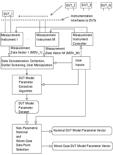
Figure 20 Using Non-Parametric Boundary Analysis—One View
The previous figure illustrates one mode of applying Non-Parametric Boundary analysis that depicts a flow of DUTs across various instrumentation interfaces. Each instrument gathers its data as dictated by the controller, which takes its inputs from the user. The gathered data is passed, in the form of a measurement data vector, into the data collection function. In the data collection block the various measurement data vectors are concatenated and manipulated. One common manipulation of the data is to discard outliers (those measurements taken from obviously defective devices, or measurements that are far removed from the prevailing data distributions). Each concatenated measurement vector is then passed to the DUT model parameter extraction algorithm. After extracting every concatenated measurement vector, a DUT model parameter data set is formed. The Non-Parametric Boundary analysis then processes the DUT model parameter data set. The result of this processing is a nominal DUT model parameter vector and a set of worst-case vectors.
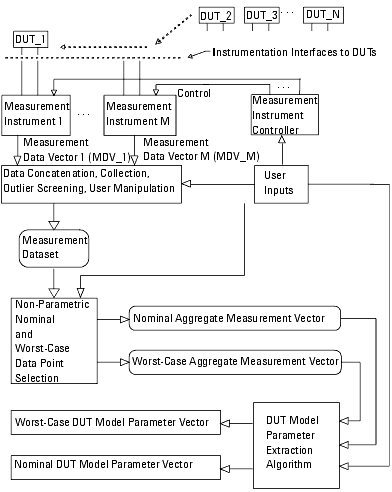
Figure 21 Using Non-Parametric Boundary Analysis—Alternate View
The previous figure shows an alternate and important variation on the data flow presented in Figure 20—the difference is the sequencing of DUT model parameter extraction. In Figure 20, the DUT model parameter extraction procedure is performed on all valid measurement data vectors drawn from the instruments, and boundary analysis is then done on the model parameter data set. Since extracting the DUT model can be computationally intense, performing the boundary analysis directly on the measurements first can lead to significantly less computing time. The flow illustrated in Figure 21 has the added benefit that the analysis is done on the electrical behavior of the DUTs. The measured electrical behavior will potentially correlate more closely to the DUT's worst-case performance in its final circuit environment. The method shown in Figure 21 is then the preferred course.
Algorithm Description
Like all algorithms, Non-Parametric Boundary analysis has inputs, outputs, and internal processes. Inputs to the Non-Parametric Boundary algorithm are:
| • | A real valued data set of S sample vectors with each vector having P parameters |
| • | B, number of boundary points |
| • | E, percent enclosed |
| • | O, diversity oversampling |
| • | D, density estimator percentage |
| • | M, distance metric |
The data set is a 2-dimensional collection of real data. Each row is a single sample with the columns containing the parameter values for each sample. The desired number of boundary points is self explanatory, as is the percent enclosed. These inputs are primary to the algorithm.
The remainder of the inputs merely influence the algorithm's behavior. Diversity oversampling allows the user some control over a process called spatial diversification. This process was developed to prevent spatial clustering of the returned boundary models. This spatial clustering manifests itself as the algorithm picking two or more boundary points that are very close to one another. The problem arises because the data set has a finite number of samples. The finite number of samples means that the raw data set exhibits clustering on some regions of the boundary. This clustering of the raw data leads to clustering of the returned boundary points.
The density estimator percentage is the percentage of sample points that are to be used as the nearest neighbors for computing density. A percentage is used (instead of an absolute number) because it is more appropriate and consequently more convenient for the user.
The outputs from the algorithm are the nominal data vector and the set of boundary vectors. It is important to note that the vectors returned are selected from the data set. This circumvents any problems with the algorithm provided data that is unrealistic.
The internal processes of the algorithm are: normalize the data set, calculate density estimates, select the nominal vector, and select the boundary vectors.
The data set must be normalized because the parameters can have vastly different magnitude ranges. Since the algorithm makes a distance calculation to estimate density, normalizing the data ensures that each parameter has equal weight in the density estimate. The data is normalized such that it is bounded by a unit hypercube. The user must perform outlier screening on the data before it is fed to the algorithm so as to ensure equal weighting of each parameter. If a given parameter naturally ranges over more than one decade of values, the user must logarithmically transform that parameter before applying Non-Parametric Boundary analysis.
The density estimate for every point in the data set is performed by finding the specified number of nearest neighbors (density estimator percentage of the number of samples) and calculating the average distance to those points. A suitable density estimate is then one over the average distance. Calculating a dimensionally correct density estimate is problematic because the Monte Carlo noise in the average distance calculation is amplified to the point that the estimate has insufficient signal to noise ratio.
Selecting the nominal point is easy—it is the point with the highest density estimate. (The algorithm returns the mode of the data.) If the data is multimodal, then the algorithm picks the mode with the highest estimated density. If there is a tie, then the returned point is arbitrarily selected between the ties.
The boundary points are selected by sorting the data points per their density estimate. The sorted data points are then partitioned into two groups. The first group includes the points with the higher density estimates. The second group includes the points with the lower density estimates. The cut between the two groups is specified such that the first group holds the enclosure percentage of the entire data set.
The boundary models are now ideally those datapoints in group one with the lowest density estimates (those points just above the cut line in the sorted list). This procedure locates a set of points for which the density estimate is approximately constant.
The final step of the algorithm is to enforce spatial diversity on the points returned. During the development of the algorithm, it became clear that the points returned were generally not evenly distributed over the boundary. The phenomena occurred for all trial validation data sets, even synthesized multidimensional Gaussian sets with a very large number of samples (>10,000). As mentioned previously, the main reason for this non-uniform spatial distribution over the boundary is that the starting data points exhibit local clustering. This situation is just a fact of life for a finite number of samples drawn from any stochastic process. The lack of spatial diversity in the boundary points arises because two or more points in a local cluster near the boundary will have nearly identical density estimates, resulting in their being adjacent in the sorted listed associated with picking the boundary points.
The spatial diversification process uses oversampling above the cut line followed by selective discarding to determine the final set of boundary points. The oversampling is done by taking some multiple of points more than the desired number of points just above the cut line. All possible pairs are formed while searching for the pair closest together. The member of the pair that is closest together and that has the higher density estimate is discarded. This process of pairing and discarding is continued until only the desired number of boundary points remain. The net result is that the points are approximately evenly distributed over the boundary.
Users will discover that three of the inputs are constrained by a formula. This formula accounts for the fact that only a finite number of points are available from which to pick the final boundary points. The formula is
int is the truncating integer operator
B is the number of requested boundary models
O is the diversity oversampling factor (1.2  0
0  5)
5)
S is the number of samples
R is a heuristic constraint on the range of density values over which boundary
models can be picked (R = 0.35)
E is the percent enclosed
The user has direct control (via the input dialog box) over B, O, and E. S is set by the provided data set. R is hardwired from the standpoint of the graphical user interface, but can be changed by modifying via a configuration file.
Algorithm Validation
A variety of methods were used to validate the functionality of the Non-Parametric Boundary analysis algorithm. Only one of these methods, 2-D scatter plots, is available in IC-CAP. The other methods were implemented in stand-alone software for the sole purpose of validation. Because there are no visualization tools for general data sets with high dimensionality, the other validation methods presented in this section use simplified data sets with specific properties.
The most obvious validation method is to take some samples from a known 2-D stochastic process and look for the expected boundary by viewing scatter plots of the samples and the selected boundary points. A good governing PDF for this stochastic process is a 2-D Gaussian. The expected boundary is then a circle or an ellipse. It is important to note that this graphical confirmation works only for a 2-D distribution. Higher numbers of dimensions require other, less direct, methods.
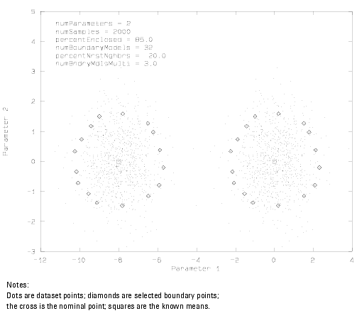
Figure 22 Scatter Plot of Bimodal Gaussian Distribution with Selected Boundary Points Overlaid
The previous figure gives an example of a 2-D scatter plot for a bimodal Gaussian distribution with the boundary points overlaid. As anticipated, the boundaries for each of the modes is approximately elliptical. Furthermore, the algorithm has no difficulty with this multimodal data. At this point, we could view a 2-D scatter plot for data distributions that are non-Gaussian. Multimodal, non-analytic distributions are the forte of this algorithm.
In higher dimensions, we employ two other validation aids. The first aid relies on making high dimensional Gaussian distributions spherical. (Set the covariance matrix for the PDF function equal to a constant times the identity matrix.) For this special type of distribution, the boundaries of constant density are shells or hypershells.
Validation proceeds by overlaying two histograms: one of the radial distance from the mean for all of the sample points and one of the radial distance to the boundary points. The expected result is for the boundary points to fall in a shell. That is, the boundary points will fall into some narrow band of histogram bins. The limitation of this tool is that the distribution must be spherical, and it must be unimodal. However, the tool works for low to modest numbers of points with any dimensionality.
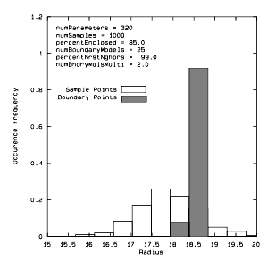
Figure 23 Overlay of Histograms of Radial Distance to Sample Points and Radial Distance to Boundary Points for a 320 Dimensional Data Set
The previous figure is an example of a radial distance histogram for a 320 dimensional data set (320 is arbitrary). Note the histogram for the entire data set is given by the unfilled bins, and the filled bin histogram is for the boundary points. The histograms indicate that boundary points do, in fact, reside in hypershell.
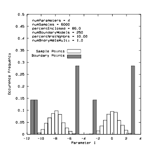
The second tool for validation in higher dimensions does not require the unimodal constraint. However, as the dimension of the space goes up, the number of sample points needed to see a result grows, probably at an exponential rate. The second tool is conditional density histograms. This tool involves taking repeated slices of the space that are parallel with each of the coordinate axes until only one dimension (independent variable) remains. A histogram is formed over some range of values for the remaining variable.
Figure 24 Conditional density histogram of a 4-D multimodal Gaussian data set
The previous figure provides a graphical affirmation of the algorithm's correct performance on a 4-D bimodal Gaussian distribution. We expect to find that the boundary points are in the tails of the two distributions—this is, in fact, what we observe.
Unfilled bins are histogram of points from entire data set that reside in the slice. Filled bins are the histogram of boundary points found in the slice. The means of the two Gaussian distributions are (-8,0,0,0) and (0,0,0,0). The covariance matrix for both distributions is the 4 x 4 identity matrix. The slice is the region of the space (-1.2 < P2 < 1.2, -1.2 < P3 < 1.2, -1.2 < P3 < 1.2), where P2, P3 and P4 are coordinate axes labels.
