Error Function Formulation

The optimizers use different methods for error function formulation. The error function formulations are shown in the following table.

Table 23 Error Function Formulation

Error Function Formulation	Optimizers
Least-squares	Levenberg-Marquardt, Gradient, Quasi-Newton, Genetic, Hybrid (Random/LM), Hybrid (Random/Quasi-Newton)
Minimax	Random Minimax, Gradient Minimax
Least Pth	Least Pth

Least-Squares Error Function (L2)

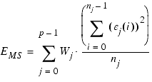
The least-squares error function (also called mean square, MS) is calculated by evaluating the error for each specified goal at each data set point individually, then squaring the magnitudes of those errors. The squared magnitudes are then averaged over the number of points.

To help you understand the error function calculation in more generality for a measurement as a function of frequency, consider the following variable definitions.

p

Total number of input columns (pair of Target and Simulated data sets) in the optimizer Inputs page. IC-CAP uses the index (j= 0, ..., p-1) to iterate between inputs.

n_j

number of data set points of the j-th input. (j = 0, ..., p-1). IC-CAP uses the index i to identify a point within the target or simulated data set.

T_j

the j-th Target data set defined in the optimizer Inputs page.

S_j

the j-th Simulated data set defined in the optimizer Inputs page.

W_j

the j-th input weighting factor as defined in the optimizer Inputs page for the j-th input.

e_j(i)

the absolute or relative error (see Relative/Absolute Error Formulation) calculated using the i-th point of the j-th Target and Simulated data sets in the optimizer Inputs page.

The total mean square error, MS is defines as:

The square root of the MS error is the well-known root mean square which is one of the optimizer termination conditions:

Minimax Error Function

The Minimax optimizer calculates the difference between the desired response and the actual response over the entire measurement parameter range of optimization. The optimizer then tries to minimize the point that constitutes the greatest difference between actual response and desired response.

Minimax means minimizing the maximum (of a set of functions generally denoted as errors). The error function is defined as the maximum among all error contributions, expressed mathematically:

among all of the i and j

where

error term e_j(i) is defined as in the previous section.

Note that the error is always positive (see Relative/Absolute Error Formulation.)

The minimax objective function always represents the worst case, where the specifications are most severely violated. The minimax optimizer will spend all its effort trying to minimize these. The goal of a minimax optimization is to meet specifications in an optimal, typically equal-ripple manner.

Least Pth Error Function

The Least P^th optimizer uses an error function formulation similar in makeup to the least squares method found in the Random, Gradient, and the Quasi-Newton optimizers. But, instead of squaring the magnitudes of the individual errors at each data set point, it raises them to the P^th power, where p = 2, 4, 8, or 16. The optimizer automatically increases p in the 2, 4, 8, or 16 sequence. This emphasizes the errors that have high values much more strongly than those that have small values. As p increases, the Least P^th error function approaches the minimax error function.

The Least P^th optimization routine is the exponential sum of the error function, where the exponent p is not necessarily equal to 2. It can be a positive number, usually an integer.

First of all, the maximum error is found as:

among all of the i and j

Since the error terms are always positive and the mimimax error EMM > 0, we can define the Least P^th error function, Epth, as follows:

The Least P^th formulation is used as an indirect method to achieve a minimax design.

Minimax error function can contain edges or discontinuities in their derivatives. These occur at points where the error contributions resulting from different goals intersect in the parameter space. The Least P^th error functions avoid this problem.

For a large value of p, the errors having the maximum value (ej(i) = E_MM) are more strongly emphasized over the other errors, i.e., they are given higher priority in optimization. As p increases to infinity, the Least P^th formulation leads to a minimax error function. The problem is solved though a sequence of Least P^th optimizations with p being gradually increased. The sequential Least P^th optimization used in the program uses p = 2, 4, 8, 16. This strategy often provides a smooth path towards a minimax solution.

For more information on the least-squares error function, refer back to Least-Squares Error Function (L2).