Performing an Optimization

The basic steps required to perform an optimization are:

1	Selecting an optimization transform.

2	Selecting an optimization algorithm.

3	Specifying the error as absolute or relative.

4	Specifying the inputs to the optimizer.

5	Specifying the parameters to be optimized.

6	Specifying the optimizer options.

7	Executing the optimization.

The following sections describe each of these steps, as well as undoing an executed optimization.

Select the Optimizer Transform

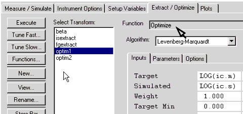
The optimizer in IC-CAP is provided in the form of a function, the Optimize transform.

To select the Optimize transform:

1	Select the setup.

2	In the Extract/Optimize folder Function data entry field, enter Optimize.

Selecting the Optimizer Algorithm

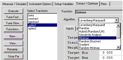
After selecting the transform, choose an algorithm from the drop-down list.

Select the Error as Absolute or Relative

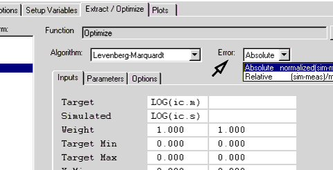
Choose an error type from the Error drop-down list.

You must specify the inputs, parameters, and options for the selected transform. The following sections describe these tables. For further details, refer to Chapter 9, "Using Transforms and Functions."

Defining Optimizer Inputs

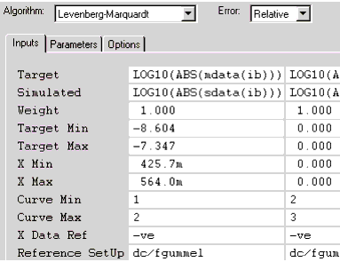
You can define the optimizer inputs by completing the Inputs table.

Figure 25 Optimizer Inputs

The fields available in the Inputs table (figure above) are:

Target

Data set containing the measured data against which simulated data is matched.

Simulated

Data set containing simulated data.

Neither target nor simulated data files must come from the same setup. The Inputs table may be used to specify either target or simulated data files from any location. The only requirement is that both data sets must have the same number of data points.

There is no limit on the number of data points.

You can also run multiple setup optimizations by entering more than one target simulated pair in the Inputs table. Enter as many target pairs as desired.

Weight

Relative weighting factor to apply to each pair of Targeted and Simulated data. For details, see Weighted Optimization.

Target Min

Lower limit for the target data values. Data values lower than this limit are ignored during optimization.

Target Max

Upper limit for the target data values. Data values higher than this limit are ignored during optimization.

X Min

Lower limit for the X-axis data values. Data with X-axis values lower than this limit are ignored during optimization.

X Max

Upper limit for the X-axis data values. Data with X-axis values higher than this limit are ignored during optimization.

Curve Min

Lower limit for the curve. For a family of curves, curves numbered lower than this limit are ignored during optimization. A single curve can be selected by entering the same curve number in both the Curve Min and Curve Max fields.

Curve Max

Upper limit for the curve. For a family of curves, curves numbered higher than this limit are ignored during optimization.

X Data Ref

Reference data set used for X boundary conditions X Min and X Max or when the variables X_LOW and X_HIGH are defined. When left blank (default), the reference data set is the first order sweep defined in the setup.

When no target or X-axis bounds are set, the bounds default to zero (0) and no bounding is performed. When minimum and maximum bound values are equal, no bounding is performed. These per-target bounds take precedence over the bounds specified in the optimizer Options table. That is, if bounds are entered in one or more Min or Max fields in an Inputs table, the bounds from the Options table are not applied to that row.

Reference SetUp

The location of the setup that all inputs will reference. When this field is left blank (default), the inputs reference the current setup.

For example, if ib.m is set as the target, ib.m must be an output or a transform in the current setup to be resolved correctly. When it points to another setup, then inputs are referenced to that setup.

You can also point to a setup in another file (for example, npn_01/dc/fgummel).

When reading, the syntax dc/fgummel is changed to ../../dc/fgummel to make it consistent with the relative path.

Defining Optimizer Parameters

You can define the parameters or variables to be optimized by completing the Parameters table. There is no limit on the number of parameters.

Figure 26 Optimizer Parameters

The settings available in the Parameters table (figure above) are:

Insert a Group

Select a group in the first Drop-down, and then all the parameters or variables defined in the group can be selected in the second Drop-down.

Insert Param or Var

No group selected in the first Drop-down, the second Drop-down list of all parameters defined in the Model Parameters table. Select a parameter to load from the Model Parameters table into the Optimizer Parameters table.

Clear Table

Select to clear values from the optimizer Parameters table.

Auto Set

Sets minimum and maximum values based on the value of the coefficient defined with the AUTOSET_COEFF variable on the System Variables page. The default coefficient value is 5.

if the Value > 0, then

Min = Value ÷ Coefficient

Max = Value × Coefficient

if the Value < 0, then

Min = Value × Coefficient

Max= Value ÷ Coefficient

if the Value =0

Min = -Coefficient

Max = +Coefficient

Using an AUTOSET_COEFF value of 5, the minimum would be set to 1/5 of the Value and the maximum would be set to 5 times the Value setting. An AUTOSET_COEFF value of 8 would result in the minimum set to 1/8 of the Value and the maximum would be set to 8 times the Value setting.

Name

Name of a model parameter, DUT parameter or variable that is to be optimized. A parameter can be removed temporarily from an optimization by placing an exclamation point (!) before its name.

Min

Minimum acceptable value of parameter.

Max

Maximum acceptable value of parameter.

Stored

The last stored value for the parameter.

The Store Par button stores the current parameter Value setting in the optimizer Parameters table to the Model Parameters table.

The Recall Par button recalls the last stored parameter Value setting in the optimizer Parameters table from the Model Parameters table.

Tuner

Sets the Tuner to linear (L) or logarithmic (G) scale for the parameter. Default is G logarithmic.

The Tune Fast and Tune Slow buttons open a tuner window. The tuner enables you to adjust the parameter values. You can see the effects in a plot as you vary parameter values using the tuner.

Tune Fast recalculates constantly as a slider is moved. Tune Slow recalculates only when a slider is released.

While the tuner window is open, you can change the Min and Max values. It's best to use Tune Slow when the time per calculation is slow (about one second or more).

Store Param

Locally stores the current parameter values to the Stored column on the Parameters table. When the file is saved, these values are stored as part of the optimizer settings.

Recall Param

Resets the Parameters table values to the locally stored values.

Defining Optimizer Options

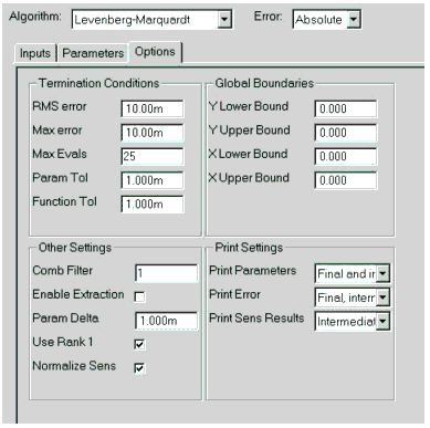
The Options table is divided into the following groups: Termination Conditions, Global Boundaries, Other Settings, and Print Settings. The specific variables contained within these four groups will change depending on the currently selected algorithm.

As an example, the following figure shows the optimizer Options table for the Levenberg-Marquardt algorithm.

Figure 27 Optimizer Options, Levenberg-Marquardt Algorithm

Termination Conditions

This group of settings determine the values at which the optimization process terminates. The following data fields may be active, depending on which algorithm is selected.

Function Tol

Optimization stops when the percentage change in RMS error value, from one optimization to the next, is less than the specified value.

Max error

Optimization stops when the maximum error between measured and simulated data is less than the specified value.

Max Evals

Optimization stops when the number of function evaluations (which normally are simulations) exceeds the specified value.

Max Iters

Optimization stops when the number of iterations reaches the specified value.

Parameter Tol

Optimization stops when the percentage change in each parameter value, from one optimization to the next, is less than the specified value.

Rand Iters

Optimization stops when the number of iterations reaches the specified value.

RMS error

Optimization stops when the RMS deviation between all measured and simulated data points is less than the specified value. Percentages are normalized to 1. For example, 1% is specified as 0.01.

Global Conditions

This group of settings determine the rectangular limitations of the optimized data set.

Y Lower Bound

Sets a lower limit for Y-axis data values. Data values lower than this limit are ignored during optimization. Bounding is performed according to the target data values. If a target data point falls within the specified range, the simulated data point is also used in the optimization, regardless of its value.

Y Upper Bound

Sets an upper limit for Y-axis data values. Data values higher than this limit are ignored during optimization.

X Lower Bound

Sets a lower limit for X-axis data values. Data values lower than this limit are ignored during optimization. X-axis bounding only applies to the main sweep of the Setup that contains the target data set. This cannot be changed by simply specifying a different X-axis on a plot.

X Upper Bound

Sets an upper limit for X-axis data values. Data values higher than this limit are ignored during optimization.

You can set these bounds by using the Y_LOW, Y_HIGH, X_LOW, and X_HIGH variables. However, any functions, such as log, that are applied to the data sets in the Inputs table must be applied to the bounds also.

When no bounds are set, the option defaults to zero (0) and no bounding is performed. Also, when upper and lower bound values are equal, no bounding is performed. These bounds are only applied to targets that do not have any per-target bounds specified. That is, if bounds are entered in one or more of the target Min/Max, X Min/Max, or curve Min/Max fields, the bounds from the Options table are not applied to that Inputs table row.

Other Settings

This group of settings determine values specific to the chosen algorithm. The following data fields may be active, depending on which algorithm is selected.

Comb Filter

Filters the target data to be used in the optimization by using every n^th point, where n is the value set in this field. For example, set the value to 2 and the optimizer uses every other data point. Set the value to 3 and the optimizer uses every third data point, and so on. The comb filter uses at least one data point from each data set.

Enable Extraction

Select checkbox when optimization is to run when Extract is selected from the DUT or Setup Menu. The optimization is performed after any extractions that are defined in the Setup have been run.

Normalize Sens

Controls the sensitivity analysis. Select check box for normalized sensitivities. Deselect checkbox for raw partial derivatives.

Param Delta

Controls the parameter delta used in the optimizer when calculating the numerical derivatives. Typically this option is not altered, but altering it may be useful for certain time domain optimizations. The default is 0.001.

Rand Std Dev

Controls the standard deviation of the Gaussian distribution for Random optimization. The default is 0.3.

Rand Reward

Specifies the reward coefficient for Random optimization. The default = 0.5.

Rand Penalty

Specifies the penalty coefficient for Random optimization. The default = 0.5.

Rand Seed

Specifies the seed that controls the initial random jump. The default = 0.

Use Rank 1

Select checkbox to allow the Broyden rank one Jacobian update.

Print Settings

This group of settings determine print values specific to the chosen algorithm. The following data fields may be active, depending on which algorithm is selected.

Print Parameters

Sets option for printing parameter data.

Print Error

Sets option for printing error data.

Print Sens Results

Sets option for printing sensitivity information.

Executing an Optimization

To perform an optimization on the active setup,

1	Select the setup.

2	Click Optimize Setup.

To perform an optimization on all setups in the active DUT,

1	Select the DUT.

2	Click Optimize DUT.

Undoing an Optimization

To undo an optimization, click the Undo Optim button on the Extract/Optimize page.

Pressing this button resets the optimized parameter values to values prior to the optimization and runs a simulation.