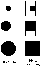
Halftoning or analog halftoning is a process that simulates shades
of gray by varying the size of tiny black dots arranged in a regular
pattern. This technique is used in printers, as well as the publishing
industry. If you inspect a photograph in a newspaper, you will
notice that the picture is composed of black dots even though
it appears to be composed of grays. This is possible because
of the spatial integration performed by our eyes. Our eyes blend
fine details and record the overall intensity [1]. Digital halftoning
is similar to halftoning in which an image is decomposed into
a grid of halftone cells. Elements (or dots that halftoning uses
in simulates shades of grays) of an image are simulated by filling
the appropriate halftone cells. The more number of black dots
in a halftone cell, the darker the cell appears. For example,
in Figure 4, a tiny dot located at the center is simulated in
digital halftoning by filling the center halftone cell; likewise,
a medium size dot located at the top-left corner is simulated
by filling the four cells at the top-left corner. The large dot
covering most of the area in the third image is simulated by filling
all halftone cells.

Three common methods for generating digital halftoning images are
Patterning is the simplest of the three techniques for generating
digital halftoning images. It generates an image that is of higher
spatial resolution than the source image. The number of halftone
cells of the output image is the same as the number of pixels
of the source image. However, each halftone cell is subdivided
into a 4x4 grid. Each input pixel value is represented by a different
number of filled squares in the halftone cell. Since a 4x4 grid
can only represents 17 different intensity levels, the source
image must be quantized. Figure 4.2 shows Rylander's recursive
patterning matrices, which will be used in listing 4.1, and a
sample of the patterning operation.


pattern - generates a digital halftoning image of the input image
via patterning.
SYNOPSIS
pattern(input_file_name, output_file_name)
DESCRIPTION
pattern generates a digital halftoning image from an input
image using the patterning technique. The program pattern
reads an input image, quantizes the pixel values, and maps each
pixel to its corresponding pattern. The resulting image is 16
times larger than the original. The generated image is written
to the output file as a TIFF file. A word of caution: "patterning"
requires a large number of computations, images of size less than
100x100 are recommended.
EXAMPLES
pattern('PAINTER.TIF', 'pa_ptr.tif')
This example generates a digital halftoning image from PAINTER
using the patterning technique (Figure 4.4)
|
|
| a. Original PAINTER | b. Digital halftoning image of PAINTER via patterning |
Figure 4.4 Digital halftoning via patterning
Another technique used for generating digital halftoning images
is dithering. Unlike patterning, dithering creates an output
image with the same number of dots as the number of pixels in
the source image. Dithering can be thought of as thresholding
the source image with a dither matrix. The matrix is laid repeatedly
over the source image. Wherever the pixel value of the image
is greater than the value in the matrix, a dot on the output image
is filled. A well-known problem of dithering is that it produces
artifacts of patterns introduced by fixed thresholding matrices.
Figure 4.5 shows a sample of the dithering operation.

Figure 4.5 The dithering operation
Listing 4.2 is a MATLAB implementation of the dithering process.
dither - generates a digital halftone image via dithering
SYNOPSIS
dither(input_file_name, output_file_name)
dither(input_file_name, output_file_name, dmatrix)
DESCRIPTION
The first synopsis uses a default dither matrix to threshold the input image. The default dither is

This matrix is a rectangle dither matrix extracted from a 450
dither matrix. 450 dither matrices can make artifacts
less obvious. The second synopsis, on the other hand, uses the
dither matrix defined by the user. dither reads in an
input image, compares each pixel with the corresponding element
in the dither matrix, generates the output image, and writes it
to the output file, which is in TIFF format. A word of caution:
since "dither" requires a large number of computations,
images of size less than 100x100 are recommended.
EXAMPLES
dither('LENA.TIF', 'di_le.tif')
This example generates a digital halftone image from LENA using
the default dither matrix (Figure 4.5a.)
dither('S_PAINTER.TIF', 'di_spa.tif', [105,135,30;90,67.5,120;45,15,45;])
This example generates a digital halftone image from PAINTER using a dither matrix defined by the user (Figure 4.5b.)
|
|
|
| a. Dithered LENA | b. Dithered PAINTER |
Figure 4.5 Examples of dithering output images
Error diffusion is another technique used for generating digital
halftoned images. It is often called spatial dithering. Error
diffusion sequentially traverses each pixel of the source image.
Each pixel is compared to a threshold. If the pixel value is
higher than the threshold, a 255 is outputted; otherwise, a 0
is outputted. The error - the difference between the input pixel
value and the output value - is dispersed to nearby neighbors.
Error diffusion is a neighborhood operation since it operates
not only on the input pixel, but also its neighbors. Generally,
neighborhood operations produce higher quality results than point
operations. Error diffusion, when compared to dithering, does
not generate those artifacts introduced by fix thresholding matrices.
However, since error diffusion requires neighborhood operations,
it is very computationally intensive.
Listing 4.3 is a MATLAB implementation of the error diffusion
algorithm
error_diffusion - generates a digital halftoned image using error
diffusion
SYNOPSIS
error_diffusion(input_file_name, output_file_name, threshold)
DESCRIPTION
error_diffusion generates a digital halftoned image using
error diffusion. It reads an input image, compares each pixel
with the input threshold, and sets the output to 0 or 255. The
quantization error is then computed and dispersed to input pixels
to the right and below the current pixel with different weights.
The weights used in this implementation were first specified
by Floyd and Steinberg (1975). Figure 4.6 shows Floyd and Steinberg's
error filter. The output image is written into the output file
in TIFF format. A word of caution: since "error_diffusion"
requires excessively intensive computations, images of size less
than 70x70 are recomended.
| threshold | --the value that determines the output to be 0 or 255. It is usually set to 128 |

EXAMPLES
error_diffusion('LENA.TIF', 'ed_le.tif', 128)
This example error diffuses LENA using 150 as the threshold (Figure
4.7a).
error_diffusion('PAINTER.TIF', 'ed_pa.tif', 150)
This example error diffuses PAINTER using 128 as the threshold
(Figure 7.6b).
|
|
| a. Error-diffused LENA | b. Error-diffused PAINTER |
Figure 4.7 Examples of error_diffusion output images