Noema: Hardware-Efficient Template Matching for Neural Population Pattern Detection
DOI: https://doi.org/10.1145/3466752.3480121
MICRO '21: MICRO-54: 54th Annual IEEE/ACM International Symposium on Microarchitecture, Virtual Event, Greece, October 2021
Repeating patterns of activity across neurons is thought to be key to understanding how the brain represents, reacts, and learns. Advances in imaging and electrophysiology allow us to observe activities of groups of neurons in real-time, with ever increasing detail. Detecting patterns over these activity streams is an effective means to explore the brain, and to detect memories, decisions, and perceptions in real-time while driving effectors such as robotic arms, or augmenting and repairing brain function. Template matching is a popular algorithm for detecting recurring patterns in neural populations and has primarily been implemented on commodity systems. Unfortunately, template matching is memory intensive and computationally expensive. This has prevented its use in portable applications, such as neuroprosthetics, which are constrained by latency, form-factor, and energy. We present Noema a dedicated template matching hardware accelerator that overcomes these limitations. Noema is designed to overcome the key bottlenecks of existing implementations: binning that converts the incoming bit-serial neuron activity streams into a stream of aggregate counts, memory storage and traffic for the templates and the binned stream, and the extensive use of floating-point arithmetic. The key innovation in Noema is a reformulation of template matching that enables computations to proceed progressively as data is received without binning while generating numerically identical results. This drastically reduces latency when most computations can now use simple, area- and energy efficient bit- and integer-arithmetic units. Furthermore, Noema implements template encoding to greatly reduce template memory storage and traffic. Noema is a hierarchical and scalable design where the bulk of its units are low-cost and can be readily replicated and their frequency can be adjusted to meet a variety of energy, area, and computation constraints.
ACM Reference Format:
Ameer M. S. Abdelhadi, Eugene Sha, Ciaran Bannon, Hendrik Steenland, and Andreas Moshovos. 2021. Noema: Hardware-Efficient Template Matching for Neural Population Pattern Detection. In MICRO-54: 54th Annual IEEE/ACM International Symposium on Microarchitecture (MICRO '21), October 18–22, 2021, Virtual Event, Greece. ACM, New York, NY, USA 13 Pages. https://doi.org/10.1145/3466752.3480121
INTRODUCTION
There are approximately 86 billion neurons in the human brain with trillions of connections. These neurons generate and transmit electrophysiological signals to communicate within and between brain regions. More than two centuries ago Galvani pioneered the study of bioelectricity using simple electrode technologies applied to the frog nerve and muscle [25]. Our understanding of the electrical currents of nerves has since greatly expanded using increasingly refined techniques [32, 34] resulting in modern neuroprobe technologies including the tetrode, Michigan silicon probes, Utah microelectrode arrays, Thomas electrodes, electrode drive mechanisms [70], and neuropixel probes [36]. More recently, genetic techniques manipulate neurons to express calcium indicators so neuron bioelectricity could be imaged [80]. Collectively, these new technologies enable us to capture the activity of ever increasing populations of neurons. Ultimately, the signals these probes capture, are digitized and processed in the digital domain.
Several challenges remain for the development of a widely accepted neuron-based brain machine interface, including electrode bio-compatibility, large-scale sampling of neuronal data, real-time pre-processing and storage of the data, “sorting” neural spike activity, detecting neural patterns, and selecting the relevant patterns [57, 69, 77]. These challenges require innovation in several disciplines. Undergoing efforts in electrode bio-compatibility include coatings [69, 76, 78], avoiding the destruction of vasculature [53], and the development of electrodes made from neural tissue itself [9]. Attempts have been made in the calcium imaging domain via some level of genetic manipulation [19]. However, invasive imaging methods tend to have better long term signal stability [10, 83], as demonstrated in animal models, and represent a real future potential for neuron detection.
As advancements in sensing technologies accelerate, the downstream digital processing stack must also grow for the overall system to keep pace. The success of such systems hinges upon meeting latency, throughput, energy, and form-factor constraints when processing the raw neural data stream. While innovations are still to occur, the algorithms employed for processing have become widely adopted and are sufficiently stable for a variety of applications. Existing implementations are predominantly in-house, most of which are only appropriate for off-line analysis on a limited number of neurons. Such implementations often fail to meet the aforementioned constraints for portable applications such as neuroprosthetics. Developing computing systems to meet the needs of current and future neuron-based brain machine interfaces can be highly inaccessible due to the need for multidisciplinary collaboration. The time and effort required to learn to “speak” the language of other fields and to hone in on the most relevant features are major up-front costs necessitating strong commitments and incentives from all parties involved. This is even more challenging when coupled with the prototype development costs of custom hardware, and its eventual deployment to scale.
As a result of such a collaborative effort, we report our experience in analyzing and developing a custom hardware platform to meet the requirements of a major component of such systems: pattern matching. The goal of pattern matching is to detect if a certain pattern of neuron activity occurs over some short period of time. This processing is purely in the digital domain, and its input are bit streams each representing the activity in time of one or more neurons. Such patterns of neuron activity are thought to be key to understanding how the brain represents, reacts, and learns from the external environment [59, 60]: Neuronal populations have been found to have reliable motor activation, replay patterns of activity in association with previous experiences during wakefulness [16, 37], sleep [20, 23, 37, 43, 46, 62, 74] and intrinsically [13, 48, 49] during field oscillation. During sleep, these patterns can recur at accelerated rates [23, 43, 46, 54], and even in reverse order [24]. The “memory” replay of these patterns can occur across various brain regions and in coordination [35, 58]. Analytic output from populations of neurons can effectively drive robotic limbs [15, 42, 50]. Taken together, detecting patterns of neuronal populations is an effective means to explore and predict the brain. Pattern matching algorithms could detect memories, decisions, emotions, perceptions in real-time while driving effectors such as robotic arms, memory retrieval or even augment brain function. As most of these applications need to be untethered, where the device can be carried by the subject with a portable power source, a small form factor and low power consumption (less than 2W [53, 66]) are highly desirable.
As we will later expand upon, the current computational and memory demands of pattern matching only worsen with the rapid increase in the number of neurons simultaneously recorded. Recent estimates range from 3,000 neurons [72] when recording with electrophysiological signals [36] to upwards of a million when recording from optical signals [39]. Accordingly, there is a growing need for accelerating algorithms and dedicated devices to process patterns of neural data fast enough for real-time applications. Pattern matching is challenging since a pattern is not an exact sequence of neuronal activity that repeats perfectly every time. Instead, pattern detection has to cope with inherently “noisy” neuron activity signals to assess patterns with some level of certainty. A range of algorithms have been used to assess patterns of activity in populations of neurons and include; Bayesian decoding [17, 29], recurrent artificial neural networks [15], explained variance [41, 74], correlations of cell pairs [16, 37] and template matching with the Pearson's Correlation Coefficient, or Template Matching for short [21, 23, 46, 51, 62, 74, 75, 79, 81]. The feasibility of a real-time pattern detection system has been demonstrated with a Bayesian decoding scheme with 128 electrodes [17, 29] while studies involving recurrent artificial neural networks relied upon 32 neuron recordings [15]. A desktop-class GPU could process 2000 channels of data input in less than 250msec [33]. Unfortunately, in real-time applications a 50msec response is highly desirable [18].
The memory and computation needs of Template Matching vary depending on the number of sampled neurons, and the number and size of the pre-recorded templates. We study representative configurations for a broad spectrum of applications (Table 1). At the lower-end are applications possible with existing commodity hardware (albeit still not portable), whereas at the high-end are applications that are not practical today but for which the neuroprobe technology is within reach. Inspired by previous work in template matching [23, 46, 62, 74] section 5 presents PCCBASE, a highly optimized vector-unit-based implementation of template matching. PCCBASE is representative of current implementations. However, our implementation optimizes memory and compute organization to best match the needs of each configuration studied, some of which far exceed previously published studies. For the configurations studied, the computation requirements vary from 600MOPS (operations, defined as an arithmetic operation) to 1.7GOPS per template. The on-chip storage of PCCBASE ranges from 40KB for our lowest-end configuration to 160MB for the most demanding one. We highlight the following observations about past implementations of template matching as motivation for our optimized design. Existing implementations of template matching implement Pearson's Correlation as originally proposed. To do so they first bin the input bit-streams of activity, into streams of aggregate integer counts. The core computation initiates only after a full time window of relevant samples (equal to the template's time dimension) has been received, impacting memory storage needs and traffic and worse response times. Many of these are floating-point computations. As section 5.4 corroborates, even desktop-class GPUs fail to meet real-time latency for more demanding applications.
As our main contribution, section 3 presents Noema, a hardware accelerator that greatly reduces area and energy costs compared to PCCBASE while maintaining real-time performance. Noema reduces costs and up-time for the configurations that are practical with PCCBASE, and supports even more demanding configurations and thus can enable further advances in neuroscience. At the core of Noema is a decomposition of the template matching algorithm where the bulk of the computations are performed using simple, low-cost, specialized bit-level operations. More importantly, in stark contrast with existing implementations, Noema performs its bulk of the computations as it receives samples bit-by-bit, producing the final output only a few cycles after the last bit in the relevant window is seen. Besides reducing latency, Noema’s approach avoids having to temporarily store the incoming stream, saving memory storage and traffic. To further reduce memory storage and traffic, we observe that templates naturally exhibit a geometric-like distribution in their value content which is heavily biased towards very low magnitude values. We equip Noema with a hardware-efficient decoder to greatly reduce template storage and traffic with little energy and area cost. For the most demanding configuration, Noema needs 34MB of on-chip storage. The simplicity and tiny area cost of the processing units of Noema enables tuning the operating frequency to improve power efficiency via partitioning and replication at a minimal area overhead (see section 3.6). We study Noema and PCCBASE as custom hardware implementations performing synthesis and layout and also summarize the characteristics of an FPGA implementation of Noema. We use our template compression for all designs. We also study the performance of our decomposed template matching implementation over commodity hardware: an embedded class general purpose processor (CPU), and a desktop class graphics processor (GPU).
This work contributes a computer-architect-targeted introduction to a typical neuroprobe processing pipeline with the emphasis being on a critical component, pattern matching, along with use cases representative of a range of applications. This introduction includes a detailed description of a popular template matching implementation and a discussion of the challenges faced by implementations over a variety of commodity platforms. These summaries motivate Noema a hardware-friendly reformulation of template matching.
We highlight the following takeaways and innovations:
- As presented and currently implemented, Pearson's Correlation requires storing the templates and a correspondingly large window of the input incoming stream in binned form. These matrices are costly, e.g., 1.24Gb each.
- The computation needs also grow and reach 1.6TOPs (mostly floating-point) for the largest configuration studied.
- Computation latency and throughput are the primary challenges as the computation has to finish within strict constraints (5 msec per window).
- Noema reformulates the computation so that the input streams are consumed as they are received bit-by-bit, obviating the need for buffering the input. This: 1) greatly reduces memory needs, and 2) allows Noema to meet real-time response times as it leaves very little computation to be done after a window's worth of input is received (throughput is now the key constraint).
- Noema’s formulation enables the use of tiny bit-serial units for the bulk of the computation. Noema replicates and places these units near the template memory banks (near memory compute). This enables high data parallel processing and scaling at low cost.
- Noema uses a hierarchical, tree-like arrangement of the compute units where floating point and expensive operations are needed sparingly.
- Noema exploits the sparsity of the template content via per bank, light-weight, hardware friendly decompression units. Templates are compressed in advance in software.
- Noema can greatly reduce power by gating accesses to the template memory, as the input bit stream is sparse and the inputs are processed a single bit at a time.
We highlight the following experimental findings:
- Noema can meet the real-time requirements: Depending on the configuration it requires 683mw to 1.2W and occupies respectively 0.11mm2 to 205mm2 in a 65nm process node.
- Noema’s template compression reduces template memory size by at least 2.79 × (most demanding conf.).
- An FPGA implementation meets real time requirement only for some of the configurations studied.
- An embedded class CPU fails real-time constraints for all configurations while a desktop class GPU fails for the most demanding ones.
BACKGROUND AND PRELIMINARIES
Figure 1 shows a high-level neural processing system for pattern detection. Using neuroprobes, electrophysiological spikes of a living brain tissue are continuously sampled and processed initially as analog signals. This spike detection and sorting stage produces a time-ordered digital stream of binary indicators (0 or 1). There is one indicator qn[t] per neuron n and per time step t. The typical sampling rate of neural spikes is 30KHz [26, 30, 56] resulting in a 30,000 bits/sec stream per neuron. Today, applications use neuroprobes capable of capturing the activity of several hundreds of neurons [36, 72]. However, the technology is rapidly evolving and neuroprobes capturing thousands and eventually millions of neuron are within sight [40, 52].
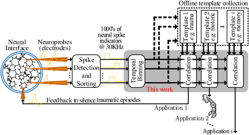
Pattern detection relies on the observation that certain events of interest such as memories, decisions, or perceptions, manifest as patterns in the neuron stream [35, 58]. Informally, as Figure 1 depicts, in these applications, patterns of interest have been pre-recorded and are continuously compared against the incoming indicator stream. Naturally, this pattern matching process is not precise and has to rely on some stochastic proximity metric. This work targets applications where pattern matching occurs in real time. Relevant applications include memory detection in real time for prosthetic control. a pattern detection latency of 50ms is desirable [18]. This is defined as the time needed to detect the pattern once receiving the very last indicator. We will use the term latency to refer to the pattern detection latency.
Template Matching
Informally, as Figure 1 shows, template matching involves sliding the incoming neuronal activity stream over a spatiotemporal template of activity indicators — a matrix corresponding to pre-recorded neural activity where rows correspond to neurons and columns to indicators over a period of time — to determine when there is a sufficient correlation. For clarity, lets assume that there is only one template. The process proceeds in parallel for multiple patterns.
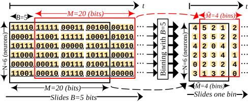
Formally, the template matching unit accepts as input: i) N digital streams of spike indicators qn[t]: n ∈ {1…N}, each being a single bit denoting if a spike from neuron n occurred at time t, and ii) a template matrix  of N rows and M columns containing pre-recorded binary indicators over a time period M. The typical sampling rate for input indicators is 30KHz [26, 30, 56]. However, the spiking rate of neurons is typically between 1Hz and 20Hz with a 1KHz maximum [45]. Using a much higher sampling rate of 30KHz provides precise temporal resolution for when spikes occur. As the indicator stream is noisy, every B indicators per neuron in the incoming stream and the template are “binned”, that is aggregated into a fixed point value of BEff ≪ B bits (defined in section 3.4). Binning occurs at runtime for the incoming stream, and off-line for the template D. B is chosen empirically to best match the resolution needed. The lower the B the higher the resolution of the observable spatiotemporal relationships, but also the noisier they become. The matching unit performs correlation once it receives M indicators. The correlation process is repeated in a sliding window fashion over the input stream, and every time another complete bin of B indicators per neuron is received. Figure 2 is an example of binning the incoming stream.
Template matching uses the Pearson's Correlation Coefficient (PCC) which is a general measure of similarity between two samples X, and Y of size L defined as:
(1)
In template matching we perform the above correlation element-wise between two binned indicator matrices: the pattern matrix D and of an equally sized window W of the incoming indicator stream matrix Q. D and W are derived from N × M × B indicators, and after binning contain elements each of lg(BEff) bits. The computational and memory needs of PCC vary greatly depending on the following four parameters: N the number of neurons, the event duration M, the resolution at which activity is to be aggregated or bin size B, and finally the number of templates T.
Multiplexing of the Indicator Streams
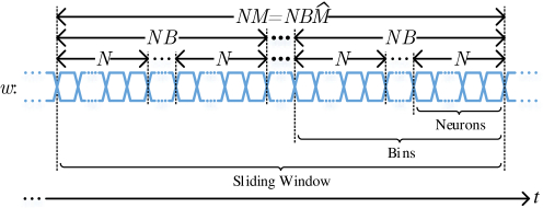
While thus far we assumed (for clarity) that there are N separate incoming streams, one per neuron, the costly analog front-end unit that generates the indicators is typically shared over multiple, if not all neurons [1, 47, 82]. As a result the analog front-end's output naturally time-multiplexes the indicators of several neurons over the same digital output serial link as Figure 3 shows. Given the relatively low acquisition rate of 30KHz per neuron a single digital serial link can easily communicate the indicators of 10s of thousands of neurons. Without loss of generality, from this point on we assume that all N neurons are serialized into a single batch of N binary indicators all corresponding to the same time step. B of those batches are read to form a complete bin, thus NB serial indicators are read as a complete bin. Similarly, bins are read to form a complete sliding window, thus serial indicators are read as a complete sliding window.
Implementation Challenges
Table 1 identifies four configurations that are representative of current and future applications as per the following best-practices in neuroscience: In accordance with previous neuroscience research demands and configurations, bin sizes range from 5 to 250msec [23, 46, 62, 74, 81] while window values range from 1 to 9sec [74]. The maximum number of neurons recorded with electrophysiology is around 3000 [72], while the number of templates may vary (and can be increased) as the use-cases demand. Accordingly, for the purpose of stress-testing, our configurations (CFG1 − 4) encompass the extreme values currently used in neuroscience (CFG1) while anticipating an increase in the number of neurons simultaneously recorded as technology evolves (CFG4). For applications that involve detecting memories (e.g., traumatic events), templates of 5 to 9 seconds (M) binned over 5 to 250 msec (B) are of interest (recall, the acquisition rate is 30KHz).
| N | T | M | B | Requirements | |||||
|---|---|---|---|---|---|---|---|---|---|
| Neurons | Templates | Samples | sec. | Bins | Samples | msec. | 0ptGOPS/Template | 100ptMemory(Mb) | |
| CFG1 | 1K | 1 | 150k | 5 | 20 | 7500 | 250 | 0.6 | 0.3 |
| CFG2 | 10K | 2 | 150k | 5 | 1000 | 150 | 5 | 314.0 | 114.4 |
| CFG3 | 20K | 3 | 270k | 9 | 36 | 7500 | 250 | 21.6 | 33.0 |
| CFG4 | 30K | 4 | 270k | 9 | 1800 | 150 | 5 | 1696.6 | 1236.0 |
The table also reports: a) the number of arithmetic operations needed over a single template and one window of the input, and b) the on-chip memory needed. The sheer volume of data and number of computations can be daunting especially for untethered applications. In real-time applications, another major challenge emerges: the bulk of the computations can be performed only after the last indicator has been received, exacerbating computation and memory needs. The hardware has to be capable of performing the computations within stringent latency constraints, and also has to buffer a window sized sample of the binned input streams which further increases memory demands. Another undesirable feature of PCC is that the bulk of the computations have to use floating point arithmetic. Coupled with the latency constraints this necessitates numerous, expensive execution units. section 5 presents an optimized vector-unit-based that implements Pearson's Correlation Coefficient as originally proposed and currently used.
Noema
This section presents Noema which overcomes the challenges of exiting PCC implementations. Central to Noema is a novel decomposition of the PCC into simple bit-level operations which section 3.1 presents. section 3.2 and section 3.3 detail the hardware implementation. section 3.4 discusses the on-chip memory required motivating the hardware efficient template encoding method presented in section 3.5. Finally, section 3.6 explains scaling in the number of neurons and templates.
Reformulating Pearson's Correlation
Recall that the PCC between two samples X and Y of length L is defined in Equation (1). Substituting the arithmetic means, squaring and rearranging the PCC equation yields:
(2)
Let D (template) and W[t] (input indicator stream window starting at time t) be respectively two matrices of indicators. Our goal is to calculate the PCC of the binned and . Recall that before binning D and W contain indicators, whereas and contain binned values where , B the number of indicators per bin, N the total number of neurons, and M the per neuron sample count in indicators of the template. Let dn, c, b and be respectively the indicators and the corresponding binned indicators of the template D and where n a neuron, c and respectively columns of the pre-binned D and the binned , and b the 3rd dimension index of the indicator matrix D that are binned together to produce the binned values of . Similarly, wn, c, b[t] () refer to the corresponding elements for the current window W[t] () matrix captured from the incoming stream.
We observe that the squared Pearson's Correlation Coefficient can be split into constants and summations:
(3)
(4)
(5)
The constants, hereafter referred to as Pearson's constants, are terms involving templates only (independent of the sliding indicator matrix ) and can be computed offline. The summations, hereafter referred to as Pearson's summations, are terms dependent on and can only be calculated at runtime, once a complete bin is received. We next detail our efficient computation of Pearson's summations based on bit-serial binary indicator arithmetic.
Implementing the Pearson's Sums
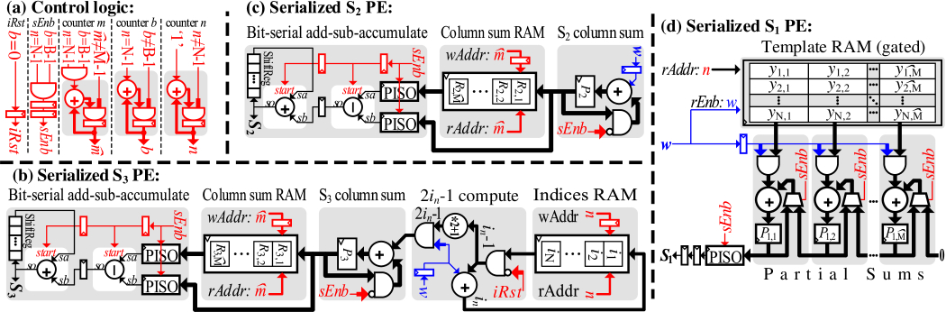
Summation S2 is the sum of all binned values in the incoming window. Since each binned value is itself a count of indicators, S2 is simply the count of all NM indicators in the window. While this count changes as the window slides, we avoid storing the whole window. As described in 1, we store the population count per column (bin) of the sliding matrix into memory R2 (6 ). Once we complete the accumulation of a new column P2 that enters to the sliding window (5 ), we add this column sum to the final S2 sum and subtract the column that exits the sliding window and was computed columns in the past (7 ).

Figure 4 (c) shows the hardware implementation of S2 PE. First, we accumulate the input indicators (received serially at w) into the S2 column sum register (P2). The control signal sEnb indicates when a column sum is ready. This happens every cycles. Once we finish accumulating a column (bin) of indicators, we move the sum P2 to the column sum memory R2 and reset P2 to prepare it for the next column accumulation. The final stage of processing S2 is the bit-serial add-sub-accumulate. This block receives the new column sum (to be added) from the column sum register P2, and the oldest column sum (to be subtracted) from the column sum memory . Both of these sums are serialized using a Parallel-Input-Serial-Output (PISO) unit, and the difference of those sums is accumulated (serially) to the final S2 value.
Summation S3, as shown in Equation (5)requires accumulating the squares of the binned input. One approach is to accumulate the binned indicators and then square the accumulated value for each bin. This is expensive as it has to accumulate values ahead of processing, and a cost-prohibitive squarer circuit for each bin of a total of N bins. Instead, we break the squares into partial sums that will be generated and accumulated as new values are received by utilizing the popular sum of first odd natural numbers equation:
(6)
Substituting in Equation (5) yields:
(7)
Where the upper bound for a is , the corresponding binned value. This summation happens on-the-fly, incrementing a every time a 1 is received. Accordingly, we do not need to know the upper bound in advance. We “discover” it naturally as the stream is received.
For efficient implementation, the summations should be organized to match the order in which the indicators are received as shown in Figure 3: in the outer summation, b in the middle summation, and n in the inner summation, namely . For this purpose, we need to keep the running indexes i for each element of the current column. This can be solved by storing intermediate copies of the variable i one per neuron n, as described in 2 .
2 is very similar to 1, however, we store a copy of the current index i of neuron n into the memory location in. in is incremented if the spike indicator w is active, and will be cleared for every n on the first bit of each the bin (5 ). The column sum P3 will be incremented by 2in − 1 if the incoming indicator w is active. This will generate the sum of squares as dictated by Equation (6).

As illustrated in Figure 4 (b), we accumulate the incoming indicators into an indices memory for each neuron of the N neurons separately, say in for neuron n ∈ {1, ⋅⋅⋅, N}. Afterwards we compute 2in − 1, and accumulate it to the column sum register P3. The computation of 2ni − 1 is performed for each neuron separately. The control signal iRst is activated every B cycles for a period of N cycle to clear the previous content of the memory. Note that we start accumulating the fragments of the squares before having the complete square value. The rest of S3 PE is similar to S2 PE.
Summation S1, as shown in Equation (5), is different than the previous two sums as it involves the template. S1 is an element-wise multiply-sum of elements from the binned template and elements from the sliding spikes matrix. The major challenge of element-wise multiply-sum that it requires recomputing all matrix elements for each incoming bin (a column in the matrices). Unlike S2 and S3 we cannot perform this summation by adding the difference between the first and the last column. However, our approach simplifies this compute-intensive operation and does not require any multiplier. We instead use an accumulator for each of the matrix columns by substituting the binned form of the input spikes sliding matrix from Equation (5) with the serialized input w. S1 will thereby be computed by:
(8)
For each of the N neurons, the binned value of the template is accumulated if the input spike indicator w is active. For instance, if the incoming spike indicators stream is “...0100101” and the current bin value is x, the value of x will be accumulated three times. The accumulators are connected in series to implement the sliding window. Once a complete bin (column) is computed (i.e., control signal sEnb is asserted), its accumulated value is moved and accumulated in the neighboring accumulator. After successive bin accumulations, all bins (columns) will be accumulated in the leftmost register. Finally, the accumulated S1 is serialized.
Post-Processing
To find the Pearson's Correlation Coefficient value, we substitute the Pearson's sums together with the pre-computed Pearson's constants into Equation (3). This computation requires (1) a constant multiplier, (2) a subtractor, (3) a squarer, and (4) a fractional divider. To reduce the overhead of the post-processing hardware, it has been implemented using traditional bit-serial arithmetic. Figure 5 illustrates a family of bit-serial arithmetic circuits that were modified to fit our needs. Our implementation exhibits a unit latency, namely, the first output bit is generated at the same cycle that the first valid bit has been received. Simply, the first valid bit propagates through a combinatorial logic to generate the first valid bit. A single register is added between each cascaded unit to break long combinatorial paths that may be created. The constant multiplier and squarer are modified versions of Gnanasekaran's carry-save add-shift semi-systolic multiplier [27]. While the aforementioned bit-serial arithmetic circuits require a control signal to indicate the last bit of bit-serial value, our modifications are only required to indicate the first bit of the bit-serial value at the beginning of the computation. This further simplifies the design. An ultra low-area fractional divider has also been implemented.

Figure 6 (b) shows the implementation of the post-processing circuitry. The post-processing unit receives bit-serial Pearson's sums, and bit-parallel Pearson's constants. Our bit-serial arithmetic units are cascaded to compute the squared PCC as formulated in Equation (3). To increase the maximum possible Fmax, we pipeline the computation together with the start signals that synchronize the computation start time for each unit. The computation performance and latency are dominated by the fractional divider, thus the post-processing units can process one set of inputs every WP cycles, where W is the data width and P is the precision of the output.
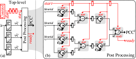
The post-processing unit has two major inputs, the Pearson's sums and the Pearson's constant. The Pearson's sums are generated serially by S1 PE, S2 PE, and S3 PE. As depicted in Figure 6, the post-processing unit receives those sums as bit-serial inputs, together with a control signal to start the processing. On the other hand, Pearson's constants are generated offline and are loaded to the post-processing unit.
On-Chip Memory Costs
Table 2 shows the cost in bits of the various storage elements given a configuration. Beff is the expected maximum count for the bin values. This maximum is a function of the intrinsic firing rate of the brain and of the sampling rate used by the analog front-end. It is known that the neurons fire at a maximum rate of 1KHz, whereas a commonly used sampling rate for neuroprobes is 30KHz (e.g. Intan technologies data acquisition system). The higher sampling rate permits a resolution that is necessary for identifying when spikes occurs. Accordingly, the expected maximum value for a binned value will not exceed B/30, where B is the total number of samples binned per value. A real example, confirmed using indicator traces from mice [71], demonstrated that for B = 150 the maximum expected value Beff = 5. As section 5.1 will show, most of Noema’s area is consumed by the template memory. Accordingly, we consider space efficient encoding of the template matrix next.
| Sub-module | Resource | Width | Depth |
|---|---|---|---|
| S1 PE | Registers (P1, PISO) | 1 | |
| Template RAM | N | ||
| S2 PE | Registers (P2, PISO, SR) | 1 | |
| Column RAM (R2) | log 2(NBeff) | ||
| S3 PE | Registers (P3, PISO, SR) | 1 | |
| Column RAM (R3) | |||
| Indices RAM (i) | log 2(Beff) | N | |
| Post-Processing | Registers | 1 |
Template Memory Compression
As Table 3 shows, the template memory size can reach hundreds of Mbits. While feasible, such memory sizes are undesirable for untethered applications. Using off-chip memory is also undesirable due to its energy and latency costs compared to using on-chip SRAM. Therefore, we explore the alternative of compressing template values on-chip.
We find that templates collected from thousands of neurons in mice [71] exhibit a geometric distribution of values, where low magnitude values dominate.Accordingly for the case of B = 150 (max binned value BEff = 5) we encode the values 0, through 5 respectively as 0b, 10b, 110b, 1110b, 11110b and 11111b. However, for larger values of B unary decoding requires large one-hot to binary decoders. Inspired by Golomb[28] and Rice[63] codes, we mix unary and binary codes to implement a simple-to-decode variable length encoding scheme referred to as UBu, b coding. A UBu, b code represents a UB code with unary variable-length codes of maximum u-bits length, and a binary fixed-length code of b-bits length. For example, for B = 7500 (max binned value BEff = 250) we use a UB4, 8 encoding. That is, values up to 3 are encoded in unary, whereas larger values are encoded with a prefix of 1111b followed by the actual value v. This encoding uses 12b in total for all values above 3. There are many other possible encoding methods that are worthwhile exploring. However, they would need to carefully balance the area, complexity, energy, and compression ratio. This is left for future work.
7a illustrates our implementation for an example UB4, 5 for clarity. To allow a single code decoding per cycle, we arrange the compression data in lines of u + b = 4 + 5 bits width. We read a single line every cycle and store the previously read line to allow processing the remaining bits from the previous line. The previous line and the current line are packed as a double-width line. The core of the decompression engine is a barrel shifter that allows reading the data from a specific starting position. After shifting the data, we know that the first u + b bits are the current code. The first u-bits are the unary part and are processed using a u-bits priority encoder to receive the index of leading zero. If all u-bits are 1’s, the current code is binary; we read the next b-bits from the binary code portion then add u to generate the decompressed data. Otherwise, the current code is unary; the output of the priority encoder (index of leading zero) is actually the decompressed data. The rest of the circuity computes the starting index of the next code and the generates the enable signal that enables reading the next line from the memory once the remainder of the combined current and previous lines is less than u + b bits. We use one decompressor unit per template memory column.
Scaling
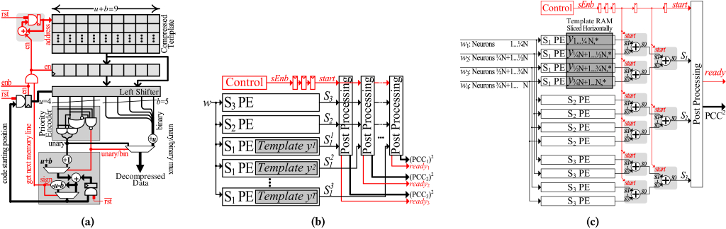
Templates: 7b shows how it can scale to support multiple templates. Fortunately, sums S2 and S3 are functions of the input stream solely. Accordingly, we need to replicate only the S1 and the post processing units.
Neurons: The first parameter available to scale up the number of neurons that Noema can process is its operating frequency. Since the units perform their computation at the same rate as the data is received, the frequency needs to be N × KHz for the design as shown to process N. To surpass the limitations of the frequency. we can scale to even more neurons by partitioning the input stream coupled with replication of the compute components as 7c shows. The example shows scaling up to 4 × more neurons by partitioning the input stream into four sub-streams, where each sub-stream is assigned its own set of sum units. The post processing unit is scaled up accordingly. The costs would be linear for the replicated sum units, whereas they are logarithmic for the post-processing unit. Fortunately, we can also simply partition the template memory, as with the input neurons. The overall area of the template memory will be mostly unaffected by the required partitioning. As the evaluation section shows, the relative cost of the processing logic in Noema is negligible compared to the template memory.
Tuning Frequency and Power: We can further reduce frequency and improve power efficiency by purposely partitioning the input stream while using more processing units. The low area needed by the compute portion of the design makes this an effective approach. Of course, care must be taken to ensure that latency remains within real-time limits. Fortunately, for the most demanding configuration we studied, the latency for producing the correlation output per window is only 700 cycles where even at a reduced clock frequency of 140KHz, Noema would still meet the 5ms requirement. Finally, by delaying the incoming stream w in Figure 4 by one cycle, Noema avoids accessing the template memory when the indicator is 0. This improves energy consumption by nearly 7X for the most demanding configuration studied as the indicator stream is sparse.
RELATED WORK
There has been no prior work on hardware accelerated PCC for processing neuronal signals for pattern matching in real time. Small scale prototype implementations of PCC routinely use commodity platforms and are computed offline.The development and implementation of new algorithms for neural decoding has been continuously expanding since 2002, when a monkey was able to move a computer cursor, directed from neural signals alone [65]. While motor prosthetics often use Kalman filters in real time, and combine them with of PCC template matching to identity events corresponding to motor memory. [21]. Accordingly, various algorithmic approaches need to be tailored to particular brain regions and the type of brain activity being detected.
In general, prior techniques for accelerating PCC can be classified along two axes. The first is the type of platform used, (1) CPUs [67], (2) GPUs [22, 38, 44], and (3) hardware-oriented techniques on FPGAs [61]. The second is the target application, where the only work on PCC acceleration has been directed at offline analysis of connectivity maps based on fMRI (blood flow) image data [61]. Thus methods for acceleration of high-resolution (i.e. neuronal signal) pattern matching remains to be investigated. Previous research on template matching in populations of neurons with the Pearson's Correlation Coefficient [23, 46, 62, 74, 75, 79, 81] has been performed with PCC and executed on commodity CPUs and GPUs operating offline, with no explicit latency constraints or focus on acceleration. Data parallelism within and across windows and batching across multiple input traces are used to maximize throughput. For real-time applications, and as section 5.4 confirms, optimized GPU implementations can meet latency constraints only for the less demanding configurations necessitating energy and latency optimized solutions such as Noema.
EVALUATION
Experimental Setup and Framework: We use actual neuron indicator streams collected over 2400 seconds from 6446 neurons of three mice, Waksman, Robbins, and Krebs [71]. For experiments requiring inputs from more neurons, we augment these traces by sampling per neuron activity from the existing trace while maintaining the overall activity factor. We perform synthesis and layout of all designs using Synopsys’ Design Compiler [73] with a TSMC 65nm technology library. We constrain the target frequency to be only as high as necessary to meet the timing requirements of each specific configuration. Layout placement and routing is performed using Cadence Innovus [14], and we estimate the power consumption in Innovus using the post-layout netlist with an activity factor of Ff, avg/Fs = 1/1500. This is the ratio between the average neuron firing rate and the sampling rate, which represents the typical neural activity factor as validated by the input datasets we use. The area and power estimation of the on-chip SRAM blocks were modeled in CACTI [31].
Optimized Baseline Implementation: Given the data parallelism, and the specific computation and dataflow patterns of PCC, we also consider PCCBASE as an alternate to Noema. PCCBASE computes the Pearson's Correlation Coefficient on binned values as it was originally proposed and implemented in highly optimized GPU implementations. PCCBASE utilizes a vector-unit-based architecture where the units have been carefully customized in count and type to perform only the various computations PCC needs and to localize communication. PCCBASE’s memory and datapath were customized to scale to the more realistic configurations avoiding centralized memory blocks, off-chip accesses and long data busses for maximum energy efficiency. We also equip PCCBASE with the same template compression method as Noema.
As Figure 8 shows, a Binning unit converts the serialized input w into the corresponding bin values per neuron. After NB cycles, the binning memory will include the value of the current bin for all N neurons. As the last N indicators are received, the bin values are finalized one per neuron per cycle. At that time, they are transferred one by one to the corresponding column in the sliding matrix unit. The sliding matrix unit contains elements each of lg(Beff) bits. Each NB cycles we choose the next column of sliding matrix and write to the corresponding segment. This will implement a sliding window of the binned spike indicators.
A set of vector processing elements (VPEs) perform the bulk of the computations needed by the correlation. For this purpose we split the correlation computation into components that can be performed over binned columns of the input (intra-column operations), and a final step that combines the per column operations to produce the final output (cross-column). The intra-column operations are computed by the VPEs. A Scalar processing element (SPE) performs the cross-column computations. Rather than allocating a VPE per template column, we split the sliding matrix column-wise into p columns where p is tuned to achieve the required acceleration.
A template unit contains T templates which it matches against the incoming stream. There are elements in the template unit each having lg(Beff) bits. For our evaluation we use the template encoding method of section 3.5 which is directly compatible with this design also. Each column of the template matrix is thereby .
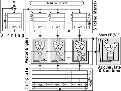
The VPEs and the SPE contain each 4x32b register files for storing their intermediate results reducing overall energy vs. using a common register file across multiple lanes. The VPE register-files are chained together to form a shift-register. This allows accumulating column data and to move the data for processing by the SPE. As a result, we have NB cycles to process the sliding matrix and to generate the PCC before the next binned column arrives and contaminates the sliding matrix content. The VPEs and the SPE implement floating-point arithmetic, as all operations with the incoming binned data as per Equation (1) entail an average. For the most demanding configuration CFG4 single-precision is needed as the individual sums in Equation (1) involve the accumulation and multiplication of 30, 000 × 18, 000 8b inputs.
We configure the number of lanes p to the minimum required to meet the 5msec latency requirement. Considering the latency in cycles per stage, we arrive at the following constraint (derivation ommitted due to space limitations):
(9)
The data range and hence datatype needs for accurate PCC calculation depend on configuration and input data distribution which in turns depend on the complexity of the spike-sorting front-end chosen and the subject/application. Our experiments show that the baseline architecture based on Equation (1) should use a single-precision FP format to avoid loss of accuracy due to accumulator saturation. Were baseline to implement the modified PCC equation Equation (2), int32 or higher could be used since the arithmetic means of the samples are not required. The scalar PE would need to still be in FP32. Compared to using a single-precision FP format to compute Equation (1), using int32 reduces the area of the vector engine by 37% and its power 43%. Taking the most intensive configuration CFG4, for example, the int32 baseline would use 12 × more power, that is an order of magnitude more power than Noema for two reasons (see section 5.2): a) the power used by the Noema PEs is 6.6 × less, and b) the baseline's template memory and buffers dominate power consuming 15.5 × more than that of Noema. In our baseline architecture we use a floating-point format since unlike integers, it won't fail for higher problem dimensions avoiding the introduction of additional complexity in applications.
On-Chip Memory
| Noema | PCCBASE | ||||||||||
|---|---|---|---|---|---|---|---|---|---|---|---|
| S1 PE | S2 PE | S3 PE | PP | Template RAM | |||||||
| Reg | Tmpl | Reg | Col. | Reg | Col. | Idx. | Reg | 5ptSlidingRAM | Uncom- | Comp- | |
| RAM | RAM | RAM | RAM | pressed | ressed | ||||||
| (Kb) | (Mb) | (b) | (Kb) | (b) | (Kb) | (Kb) | (Kb) | (Mb) | (Mb) | (Mb) | |
| CFG1 | 0.6 | 0.08 | 77 | 0.35 | 108 | 0.51 | 7.81 | 1.7 | 0.15 | 0.15 | 0.08 |
| CFG2 | 27.3 | 31.10 | 73 | 15.63 | 82 | 17.58 | 29.30 | 2.0 | 57.22 | 57.22 | 31.10 |
| CFG3 | 1.3 | 5.89 | 95 | 0.81 | 127 | 1.09 | 156.25 | 2.2 | 16.48 | 16.48 | 5.89 |
| CFG4 | 53.3 | 220.70 | 80 | 31.64 | 89 | 35.16 | 87.89 | 2.2 | 617.98 | 617.98 | 220.70 |
Template memory dominates area for the higher-end configurations. Recall, that without template compression, the capacity needed is a function of , N, and BEff. As this section shows however, compression can greatly reduce template footprints and thus the on-chip memory needed. Accordingly, before we can evaluate the ASIC and FPGA implementations, we first determine the size of the on-chip section 5.1 template memory each configuration would need.
Figure 9 reports the memory footprint for the four configurations of Table 1 and different templates with and without template compression. All footprints are normalized to the footprint of the uncompressed template per configuration. We show results for three different templates per input sample trace; a worst case which is the frame from the neuron recording with the least sparsity, and two templates which are randomly selected windows. The worst case template dictates the compression ratio used to size the on-chip template memory.
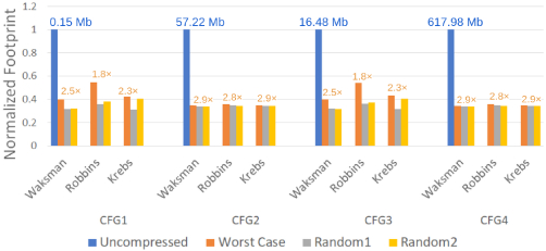
As expected, uncompressed footprint templates vary considerably, from 150Kb for CFG1 to more than 600Mb for CFG4. Our lightweight lossless compression method is effective in reducing footprints, and more so where it matters the most. That is for CFG2 () and CGF4 () configurations where footprints are reduced by at least 2.79 × for all templates. We size our on-chip memories for the worst case across the three templates per configuration. The resulting template memory sizes are shown in Table 3. The table also reports the number of bits used by the various registers per unit in Noema and the total on-chip memory needed by PCCBASE. While PCCBASE can benefit from template compression for its own template memory, it still needs a window memory for the incoming indicator streams. As we show, the ASIC implementation of Noema meets real-time requirements for all configurations and, as expected, requires considerably less power than the FPGA implementation.
Performance, Power, and Area
Table 4 shows the performance of Noema and PCCBASE in terms of throughput (number of correlations computed per second) and latency (time from arrival of last data bit to complete computation) for the four configurations. All designs are configured to meet the throughput and latency requirements. For CFG2 through CFG4 we use three partitions, each processing 1/3 of the neurons as per section 3.6. Noema far exceeds the real-time latency requirements, as it requires just 700 cycles to produce its output once the last indicator for a window is received.
| Throughput (PCC/sec) | Detection Latency (msec) | |||||||
| CFG | 1 | 2 | 3 | 4 | 1 | 2 | 3 | 4 |
| PCCBASE | 4 | 400 | 12 | 800 | 0.74 | 4.98 | 4.71 | 5.00 |
| Noema | 4 | 400 | 12 | 800 | 0.0239 | 0.0028 | 0.0015 | 0.001 |
Table 5 shows the power usage of Noema and PCCBASE for the four configurations, including a breakdown in memory and compute. Noema’s power is considerably lower than that of PCCBASE for all configurations for three reasons: 1) Noema does not need a sliding window memory, 2) the compute units are much more energy efficient, and 3) Noema can avoid accessing the template memory when a bit indicator is 0 (most will be 0 due to the nature of brain activity). PCCBASE can only exploit sparsity of binned values instead. In PCCBASE compute units are responsible for a significant fraction of overall power for all configurations, This is not the case for Noema where memory dominates total power.
| PCCBASE | Noema | |||||
|---|---|---|---|---|---|---|
| Memory | Compute | Total | Memory | Compute | Total | |
| CFG1 | 7.87 | 17.34 | 25.22 | 0.30 | 0.43 | 0.73 |
| CFG2 | 1236.74 | 607.29 | 1844.03 | 89.78 | 84.28 | 174.06 |
| CFG3 | 198.94 | 81.12 | 280.06 | 18.55 | 9.68 | 28.23 |
| CFG4 | 10718.07 | 6550.65 | 17268.72 | 682.70 | 522.76 | 1205.46 |
| PCCBASE | Noema | |||||
|---|---|---|---|---|---|---|
| Memory | Compute | Total | Memory | Compute | Total | |
| CFG1 | 0.38 | 0.15 | 0.53 | 0.10 | 0.02 | 0.11 |
| CFG2 | 81.50 | 5.87 | 87.37 | 28.46 | 1.35 | 29.81 |
| CFG3 | 15.60 | 0.77 | 16.37 | 6.26 | 0.09 | 6.25 |
| CFG4 | 469.42 | 63.48 | 532.90 | 202.00 | 3.42 | 205.42 |
Table 6 reports the area in mm2 for Noema and PCCBASE as configured to meet the real-time requirements of the four configurations. The table also shows a breakdown in the area used for memory and compute component. Noema is considerably smaller than PCCBASE. Since that all designs use our template compression, the savings with Noema are due to: 1) eliminating the sliding window memory, and 2) from using much smaller bit-serial compute units. For the CFG4 configuration, Noema is nearly 2.6 × smaller than PCCBASE. Using a more recent technology node would significantly reduce overall area. SRAM cells in a 14nm process can be 6 × to 8 × smaller compared to 65nm [11, 55, 64, 68].
FPGA Implementation
We implement Noema on a Stratix 10 FPGA (1SG280LN2F43E1VG) [4] using Intel's Quartus compiler [3]. To minimize power, the target frequency is constrained to be only as high as necessary to meet the performance requirements per configuration. Table 7 reports the resulting power, the Fmax achieved, and the minimum Fmax (Target) required to meet the real-time requirements of each configuration. The achieved latency passes real-time constraints for , but fails for . Furthermore, since the dynamic power consumed is highly correlated with the size of a template, CFG demonstrate drastic increases.
| Fmax (MHz) | Power (mW) | ||||
|---|---|---|---|---|---|
| Achieved | Target | Static | Dynamic | Total | |
| CFG1 | 467.51 | 30 | 5850.08 | 54.04 | 5904.12 |
| CFG2 | 318.47 | 300 | 5860.47 | 1016.38 | 6876.85 |
| CFG3 | 324.78 | 600 | 5851.42 | 495.03 | 6346.45 |
| CFG4 | 258.53 | 900 | 5889.82 | 12014.81 | 17904.63 |
Commodity Platforms: CPU and GPU
Software implementations of the PCC algorithm were implemented on a Raspberry Pi 3 Model B [8], an 8th generation Intel i5 laptop CPU [2] with 8 GB RAM, and NVIDIA's Jetson Nano and GTX1080 GPUs [5, 7]. The CPU implementation uses a software pipeline to perform the binning and PCC calculations as per section 3.1. Multiple configurations of data arrangements were tested with compiler flags set to infer SIMD operations where possible, and the best performing configuration was selected. Runtime and power usage are measured using an in-application timer and external power meter, respectively.
| Device | CFG1 | CFG2 | CFG3 | CFG4 |
|---|---|---|---|---|
| PCC Decomposition of Sections 3.1- 3.2 | ||||
| RPi3B | 613 | 1455 | 12240 | 112952 |
| i5 7000 | 63 | 257 | 1260 | 8605 |
| GTX1080 - Manual | 0.28 | 26.67 | 5.36 | 274.1 |
| Jetson Nano - Manual | 4.4 | 77.2 | * | * |
| Original PCC Formulation | ||||
| GTX1080 - Thrust | 1.20 | 4.27 | 3.96 | 20.6 |
| Jetson Nano - Thrust | 2.26 | 196 | * | * |
| GTX1080 - Fast-GPU-PCC [22] | 167.2 | 619.9 | 522.2 | 11395 |
Multiple GPU implementations were evaluated on the Jetson Nano and GTX1080. The first was a hand-tuned implementation utilizing the same PCC decomposition and optimizations as in the CPU implementation. This performed the best for small configurations (e.g., CFG1) reflective of current use cases. The second implementation follows the original formulation of PCC. It utilizes the Thrust (v1.8.3) library [12]. On the GTX1080, it outperforms the hand-tuned version in larger configurations (CFG2 − 4) but still fails to meet real-time expectations for CFG4. However, given the GPU's size and power consumption (10W/180W, respectively) [5, 6], an embedded solution would still be impractical. The last solution used the Fast-GPU-PCC algorithm [22] which converts PCC computation into a matrix multiplication problem. The parameters are emulated by substituting the number of voxels for neurons, and the length of time for the number of bins. The algorithm performs poorly even on the GTX1080, likely due to the differences in the problem setup. For all GPU solutions, we optimistically exclude the time needed to perform binning.
Table 8 summarizes the results. Both CPUs fail real-time latency needs for CFG1 − 4, as does Fast-GPU-PCC. Raspberry Pi power was consistently measured at 2.4W, varying by < 0.1 W. Achieving real-time latency of 5ms would require an improvement of 123 × for CFG1 and of 22, 590 × for CFG4. The laptop CPU performs significantly better, but still fails to meet latency requirements by a large margin. The desktop GPU can meet real-time requirements for CFG1 − 3, but ultimately fails for CFG4 by 4 ×. More recent GPUs would improve latency, however: a) energy would remain prohibitive, and b) PCCBASE is a highly optimized GPU-like design which is more efficient for the particular application.
This work was supported by an NSERC Discovery Grant and the NSERC COHESA Strategic Research Network. The University of Toronto maintains all rights to the technologies described.
- [n. d.]. Intan Technologies LLC, RHD2000 Series Digital Electrophysiology Interface Chips. http://intantech.com/files/Intan_RHD2000_series_datasheet.pdfl. Accessed: 2020-11-17.
- [n. d.]. Intel Intel®Core™i5-8265U Processor. https://ark.intel.com/content/www/us/en/ark/products/149088/intel-core-i5-8265u-processor-6m-cache-up-to-3-90-ghz.html. Accessed: 2020-6-18.
- [n. d.]. Intel Quartus Prime Overview. https://www.intel.ca/content/www/ca/en/software/programmable/quartus-prime/overview.html. Accessed: 2020-4-17.
- [n. d.]. Intel Stratix 10 Product Table. https://www.intel.ca/content/dam/www/programmable/us/en/pdfs/literature/pt/stratix-10-product-table.pdf. Accessed: 2020-4-17.
- [n. d.]. NVIDIA GEFORCE GTX 1080. https://www.nvidia.com/en-sg/geforce/products/10series/geforce-gtx-1080/. Accessed: 2020-4-16.
- [n. d.]. NVIDIA Jetson Linux Developer Guide (32.5 Release). https://docs.nvidia.com/jetson/l4t/index.html#page/Tegra%20Linux%20Driver%20Package%20Development%20Guide/power_management_nano.html#wwpID0E0FL0HA. Accessed: 2021-6-20.
- [n. d.]. NVIDIA Jetson Nano. https://www.nvidia.com/en-us/autonomous-machines/embedded-systems/jetson-nano/education-projects/. Accessed: 2021-6-20.
- [n. d.]. RaspberryPi.org Raspberry Pi 3 Model B. https://www.raspberrypi.org/products/raspberry-pi-3-model-b/. Accessed: 2020-4-15.
- Dayo O. Adewole, Laura A. Struzyna, Justin C. Burrell, James P. Harris, Ashley D. Nemes, Dmitriy Petrov, Reuben H. Kraft, H. Isaac Chen, Mijail D. Serruya, John A. Wolf, and D. Kacy Cullen. 2021. Development of optically controlled “living electrodes” with long-projecting axon tracts for a synaptic brain-machine interface. Science Advances 7, 4 (2021). https://doi.org/10.1126/sciadv.aay5347 arXiv:https://advances.sciencemag.org/content/7/4/eaay5347.full.pdf
- Amos Arieli, Amiram Grinvald, and Hamutal Slovin. 2002. Dural substitute for long-term imaging of cortical activity in behaving monkeys and its clinical implications. Journal of Neuroscience Methods 114, 2 (2002), 119–133. https://doi.org/10.1016/S0165-0270(01)00507-6
- F. Arnaud, F. Boeuf, F. Salvetti, D. Lenoble, F. Wacquant, C. Regnier, P. Morin, N. Emonet, E. Denis, J. C. Oberlin, D. Ceccarelli, P. Vannier, G. Imbert, A. Sicard, C. Perrot, O. Belmont, I. Guilmeau, P. O. Sassoulas, S. Delmedico, R. Palla, F. Leverd, A. Beverina, V. DeJonghe, M. Broekaart, L. Pain, J. Todeschini, M. Charpin, Y. Laplanche, D. Neira, V. Vachellerie, B. Borot, T. Devoivre, N. Bicais, B. Hinschberger, R. Pantel, N. Revil, C. Parthasarathy, N. Planes, H. Brut, J. Farkas, J. Uginet, P. Stolk, and M. Woo. 2003. A functional 0.69 /spl mu/m/sup 2/ embedded 6T-SRAM bit cell for 65 nm CMOS platform. In 2003 Symposium on VLSI Technology. Digest of Technical Papers (IEEE Cat. No.03CH37407). 65–66. https://doi.org/10.1109/VLSIT.2003.1221088
- Nathan Bell and Jared Hoberock. 2012. Thrust. 359–371. https://doi.org/10.1016/B978-0-12-385963-1.00026-5
- Edgar J. BermudezContreras, Andrea Gomez Palacio Schjetnan, Arif Muhammad, Peter Bartho, Bruce L. McNaughton, Bryan Kolb, Aaron J. Gruber, and Artur Luczak. 2013. Formation and reverberation of sequential neural activity patterns evoked by sensory stimulation are enhanced during cortical desynchronization. Neuron (2013). https://doi.org/10.1016/j.neuron.2013.06.013
- Cadence. [n. d.]. Innovus Implementation System. https://www.cadence.com/content/cadence-www/global/en_US/home/tools/digital-design-and-signoff/hierarchical-design-and-floorplanning/innovus-implementation-system.html.
- John K. Chapin, Karen A. Moxon, Ronald S. Markowitz, and Miguel A.L. Nicolelis. 1999. Real-time control of a robot arm using simultaneously recorded neurons in the motor cortex. Nature Neuroscience (1999). https://doi.org/10.1038/10223
- Sen Cheng and Loren M. Frank. 2008. New Experiences Enhance Coordinated Neural Activity in the Hippocampus. Neuron (2008). https://doi.org/10.1016/j.neuron.2007.11.035
- Davide Ciliberti, Frédéric Michon, and Fabian Kloosterman. 2018. Real-time classification of experience-related ensemble spiking patterns for closed-loop applications. eLife (2018). https://doi.org/10.7554/eLife.36275
- Davide Ciliberti, Frédéric Michon, and Fabian Kloosterman. 2018. Real-time classification of experience-related ensemble spiking patterns for closed-loop applications. eLife (Oct 2018). https://doi.org/10.7554/eLife.36275
- Kelly Clancy, Aaron Koralek, Rui Costa, Daniel Feldman, and Jose Carmena. 2014. Volitional modulation of optically recorded calcium signals during neuroprosthetic learning. Nature neuroscience 17 (04 2014). https://doi.org/10.1038/nn.3712
- Kamran Diba and György Buzsáki. 2007. Forward and reverse hippocampal place-cell sequences during ripples. Nature Neuroscience (2007). https://doi.org/10.1038/nn1961
- Jean-Baptiste Eichenlaub, Beata Jarosiewicz, Jad Saab, Brian Franco, Jessica Kelemen, Eric Halgren, Leigh R. Hochberg, and Sydney S. Cash. 2020. Replay of Learned Neural Firing Sequences during Rest in Human Motor Cortex. Cell Reports 31, 5 (2020), 107581. https://doi.org/10.1016/j.celrep.2020.107581
- Taban Eslami and Fahad Saeed. 2018. Fast-GPU-PCC: A GPU-Based Technique to Compute Pairwise Pearson's Correlation Coefficients for Time Series Data – fMRI Study. High-Throughput 7, 2 (2018). https://doi.org/10.3390/ht7020011
- David R. Euston, Masami Tatsuno, and Bruce L. McNaughton. 2007. Fast-forward playback of recent memory sequences in prefrontal cortex during sleep. Science (2007). https://doi.org/10.1126/science.1148979
- David J. Foster and Matthew A. Wilson. 2006. Reverse replay of behavioural sequences in hippocampal place cells during the awake state. Nature (2006). https://doi.org/10.1038/nature04587
- Luigi Galvani. 1791. Aloysii Galvani De viribus electricitatis in motu musculari commentarius. https://doi.org/10.5479/sil.324681.39088000932442
- Yasser Ghanbari, Panos Papamichalis, and Larry Spence. 2009. Robustness of neural spike sorting to sampling rate and quantization bit depth. 2009 16th International Conference on Digital Signal Processing (Jul 2009), 1–6. https://doi.org/10.1109/ICDSP.2009.5201163
- R. Gnanasekaran. 1985. A Fast Serial-Parallel Binary Multiplier. IEEE Trans. Comput. 34, 08 (aug 1985), 741–744. https://doi.org/10.1109/TC.1985.1676620
- S. Golomb. 1966. Run-length encodings (Corresp.). IEEE Transactions on Information Theory 12, 3 (1966), 399–401. https://doi.org/10.1109/TIT.1966.1053907
- Igor Gridchyn, Philipp Schoenenberger, Joseph O'Neill, and Jozsef Csicsvari. 2020. Assembly-Specific Disruption of Hippocampal Replay Leads to Selective Memory Deficit.Neuron (2020). https://doi.org/10.1016/j.neuron.2020.01.021
- Reid R Harrison. 2008. The design of integrated circuits to observe brain activity. Proc. IEEE 96, 7 (2008), 1203–1216.
- HewlettPackard. [n. d.]. CACTI. https://github.com/HewlettPackard/cacti.
- A. L. Hodgkin and A. F. Huxley. 1939. Action potentials recorded from inside a nerve fibre [8]. Nature (1939). https://doi.org/10.1038/144710a0
- Sile Hu, Davide Ciliberti, Andres D. Grosmark, Frédéric Michon, Daoyun Ji, Hector Penagos, György Buzsáki, Matthew A. Wilson, Fabian Kloosterman, and Zhe Chen. 2018. Real-Time Readout of Large-Scale Unsorted Neural Ensemble Place Codes. Cell Reports 25, 10 (2018), 2635 – 2642.e5. https://doi.org/10.1016/j.celrep.2018.11.033
- David H. Hubel. 1957. Tungsten microelectrode for recording from single units. Science (1957). https://doi.org/10.1126/science.125.3247.549
- Daoyun Ji and Matthew A. Wilson. 2007. Coordinated memory replay in the visual cortex and hippocampus during sleep. Nature Neuroscience (2007). https://doi.org/10.1038/nn1825
- James J. Jun, Nicholas A. Steinmetz, Joshua H. Siegle, Daniel J. Denman, Marius Bauza, Brian Barbarits, Albert K. Lee, Costas A. Anastassiou, Alexandru Andrei, Çağatay Aydin, Mladen Barbic, Timothy J. Blanche, Vincent Bonin, João Couto, Barundeb Dutta, Sergey L. Gratiy, Diego A. Gutnisky, Michael Häusser, Bill Karsh, Peter Ledochowitsch, Carolina Mora Lopez, Catalin Mitelut, Silke Musa, Michael Okun, Marius Pachitariu, Jan Putzeys, P. Dylan Rich, Cyrille Rossant, Wei Lung Sun, Karel Svoboda, Matteo Carandini, Kenneth D. Harris, Christof Koch, John O'Keefe, and Timothy D. Harris. 2017. Fully integrated silicon probes for high-density recording of neural activity. Nature 551, 7679 (2017), 232–236. https://doi.org/10.1038/nature24636
- Mattias P. Karlsson and Loren M. Frank. 2009. Awake replay of remote experiences in the hippocampus. Nature Neuroscience (2009). https://doi.org/10.1038/nn.2344
- E. Kijsipongse, S. U-ruekolan, C. Ngamphiw, and S. Tongsima. 2011. Efficient large Pearson correlation matrix computing using hybrid MPI/CUDA. In 2011 Eighth International Joint Conference on Computer Science and Software Engineering (JCSSE). 237–241.
- Tony Hyun Kim, Yanping Zhang, Jérôme Lecoq, Juergen C. Jung, Jane Li, Hongkui Zeng, Cristopher M. Niell, and Mark J. Schnitzer. 2016. Long-Term Optical Access to an Estimated One Million Neurons in the Live Mouse Cortex. Cell Reports (2016). https://doi.org/10.1016/j.celrep.2016.12.004
- Tony Hyun Kim, Yanping Zhang, Jérôme Lecoq, Juergen C. Jung, Jane Li, Hongkui Zeng, Cristopher M. Niell, and Mark J. Schnitzer. 2016. Long-Term Optical Access to an Estimated One Million Neurons in the Live Mouse Cortex. Cell Rep. 17, 12 (Dec 2016), 3385–3394. https://doi.org/10.1016/j.celrep.2016.12.004
- Hemant S. Kudrimoti, Carol A. Barnes, and Bruce L. McNaughton. 1999. Reactivation of hippocampal cell assemblies: Effects of behavioral state, experience, and EEG dynamics. Journal of Neuroscience(1999). https://doi.org/10.1523/jneurosci.19-10-04090.1999
- M A Lebedev, J M Carmena, and M A Nicolelis. 2003. Directional tuning of frontal and parietal neurons during operation of brain - machine interface.Society for Neuroscience Abstract Viewer and Itinerary Planner (2003).
- Albert K. Lee and Matthew A. Wilson. 2002. Memory of sequential experience in the hippocampus during slow wave sleep. Neuron (2002). https://doi.org/10.1016/S0896-6273(02)01096-6
- Meimei Liang, Futao Zhang, Gulei Jin, and Jun Zhu. 2015. FastGCN: A GPU Accelerated Tool for Fast Gene Co-Expression Networks. PLOS ONE 10, 1 (01 2015), 1–11.
- Bengt Ljungquist, Per Petersson, Anders J. Johansson, Jens Schouenborg, and Martin Garwicz. 2018. A Bit-Encoding Based New Data Structure for Time and Memory Efficient Handling of Spike Times in an Electrophysiological Setup. Neuroinformatics 16, 2 (Apr 2018), 217–229. https://doi.org/10.1007/s12021-018-9367-z arXiv:29508123
- Kenway Louie and Matthew A. Wilson. 2001. Temporally structured replay of awake hippocampal ensemble activity during rapid eye movement sleep. Neuron (2001). https://doi.org/10.1016/S0896-6273(01)00186-6
- Song Luan, Ian Williams, Michal Maslik, Yan Liu, Felipe de Carvalho, Andrew Jackson, Rodrigo Quian Quiroga, and Timothy G. Constandinou. 2017. Compact Standalone Platform for Neural Recording with Real-Time Spike Sorting and Data Logging. bioRxiv (2017). https://doi.org/10.1101/186627 arXiv:https://www.biorxiv.org/content/early/2017/09/22/186627.1.full.pdf
- Artur Luczak, Peter Barthó, and Kenneth D. Harris. 2009. Spontaneous Events Outline the Realm of Possible Sensory Responses in Neocortical Populations. Neuron (2009). https://doi.org/10.1016/j.neuron.2009.03.014
- Jason N. MacLean, Brendon O. Watson, Gloster B. Aaron, and Rafael Yuste. 2005. Internal dynamics determine the cortical response to thalamic stimulation. Neuron (2005). https://doi.org/10.1016/j.neuron.2005.09.035
- E. M. Maynard, N. G. Hatsopoulos, C. L. Ojakangas, B. D. Acuna, J. N. Sanes, R. A. Normann, and J. P. Donoghue. 1999. Neuronal interactions improve cortical population coding of movement direction. Journal of Neuroscience(1999). https://doi.org/10.1523/jneurosci.19-18-08083.1999
- Ethan M Meyers, Mia Borzello, Winrich A Freiwald, and Doris Tsao. 2015. Intelligent information loss: the coding of facial identity, head pose, and non-face information in the macaque face patch system. Journal of Neuroscience 35, 18 (2015), 7069–7081.
- Robbin A. Miranda, William D. Casebeer, Amy M. Hein, Jack W. Judy, Eric P. Krotkov, Tracy L. Laabs, Justin E. Manzo, Kent G. Pankratz, Gill A. Pratt, Justin C. Sanchez, Douglas J. Weber, Tracey L. Wheeler, and Geoffrey S.F. Ling. 2015. DARPA-funded efforts in the development of novel brain-computer interface technologies. Journal of Neuroscience Methods 244 (2015), 52 – 67. https://doi.org/10.1016/j.jneumeth.2014.07.019 Brain Computer Interfaces; Tribute to Greg A. Gerhardt.
- Elon Musk and Neuralink. 2019. An integrated brain-machine interface platform with thousands of channels. bioRxiv (2019). https://doi.org/10.1101/703801 arXiv:https://www.biorxiv.org/content/early/2019/08/02/703801.full.pdf
- Z Nadasdy, H Hirase, A Czurko, J Csicsvari, and G Buzsaki. 1999. Replay and time compression of recurring spike sequences in the hippocampus [In Process Citation]. J Neurosci (1999).
- S. Natarajan, M. Agostinelli, S. Akbar, M. Bost, A. Bowonder, V. Chikarmane, S. Chouksey, A. Dasgupta, K. Fischer, Q. Fu, T. Ghani, M. Giles, S. Govindaraju, R. Grover, W. Han, D. Hanken, E. Haralson, M. Haran, M. Heckscher, R. Heussner, P. Jain, R. James, R. Jhaveri, I. Jin, H. Kam, E. Karl, C. Kenyon, M. Liu, Y. Luo, R. Mehandru, S. Morarka, L. Neiberg, P. Packan, A. Paliwal, C. Parker, P. Patel, R. Patel, C. Pelto, L. Pipes, P. Plekhanov, M. Prince, S. Rajamani, J. Sandford, B. Sell, S. Sivakumar, P. Smith, B. Song, K. Tone, T. Troeger, J. Wiedemer, M. Yang, and K. Zhang. 2014. A 14nm logic technology featuring 2nd-generation FinFET, air-gapped interconnects, self-aligned double patterning and a 0.0588 μm2 SRAM cell size. In 2014 IEEE International Electron Devices Meeting. 3.7.1–3.7.3. https://doi.org/10.1109/IEDM.2014.7046976
- Joaquin Navajas, Deren Y Barsakcioglu, Amir Eftekhar, Andrew Jackson, Timothy G Constandinou, and Rodrigo Quian Quiroga. 2014. Minimum requirements for accurate and efficient real-time on-chip spike sorting. Journal of neuroscience methods 230 (2014), 51–64.
- Arto Nurmikko, David Borton, and Ming Yin. 2016. Wireless Neurotechnology for Neural Prostheses. John Wiley & Sons, Ltd, Chapter 5, 123–161. https://doi.org/10.1002/9781118816028.ch5 arXiv:https://onlinelibrary.wiley.com/doi/pdf/10.1002/9781118816028.ch5
- H. Freyja Ólafsdóttir, Francis Carpenter, and Caswell Barry. 2016. Coordinated grid and place cell replay during rest. Nature Neuroscience (2016). https://doi.org/10.1038/nn.4291
- Stefano Panzeri, Jakob H. Macke, Joachim Gross, and Christoph Kayser. 2015. Neural population coding: Combining insights from microscopic and mass signals. Trends in Cognitive Sciences(2015). https://doi.org/10.1016/j.tics.2015.01.002
- Alexandre Pouget, Peter Dayan, and Richard Zemel. 2000. Information processing with population codes. Nature Reviews Neuroscience(2000). https://doi.org/10.1038/35039062
- E. Reggiani, E. D'Arnese, A. Purgato, and M. D. Santambrogio. 2017. Pearson Correlation Coefficient Acceleration for Modeling and Mapping of Neural Interconnections. In 2017 IEEE International Parallel and Distributed Processing Symposium Workshops (IPDPSW). 223–228.
- Sidarta Ribeiro, Damien Gervasoni, Ernesto S. Soares, Yi Zhou, Shih Chieh Lin, Janaina Pantoja, Michael Lavine, and Miguel A.L. Nicolelis. 2004. Long-lasting novelty-induced neuronal reverberation during slow-wave sleep in multiple forebrain areas. PLoS Biology (2004). https://doi.org/10.1371/journal.pbio.0020024
- R. Rice and J. Plaunt. 1971. Adaptive Variable-Length Coding for Efficient Compression of Spacecraft Television Data. IEEE Transactions on Communication Technology 19, 6(1971), 889–897. https://doi.org/10.1109/TCOM.1971.1090789
- B. Rooseleer, S. Cosemans, and W. Dehaene. 2011. A 65 nm, 850 MHz, 256 kbit, 4.3 pJ/access, ultra low leakage power memory using dynamic cell stability and a dual swing data link. In 2011 Proceedings of the ESSCIRC (ESSCIRC). 519–522. https://doi.org/10.1109/ESSCIRC.2011.6044936
- Mijail D. Serruya, Nicholas G. Hatsopoulos, Liam Paninski, Matthew R. Fellows, and John P. Donoghue. 2002. Instant neural control of a movement signal. Nature 416, 6877 (2002), 141–142. https://doi.org/10.1038/416141a
- Robert K Shepherd. 2016. Neurobionics: The biomedical engineering of neural prostheses. John Wiley & Sons.
- P. Socha, V. Miškovský, H. Kubátová, and M. Novotný. 2017. Optimization of Pearson correlation coefficient calculation for DPA and comparison of different approaches. In 2017 IEEE 20th International Symposium on Design and Diagnostics of Electronic Circuits Systems (DDECS). 184–189.
- T. Song, W. Rim, J. Jung, G. Yang, J. Park, S. Park, K. Baek, S. Baek, S. Oh, J. Jung, S. Kim, G. Kim, J. Kim, Y. Lee, K. S. Kim, S. Sim, J. S. Yoon, and K. Choi. 2014. 13.2 A 14nm FinFET 128Mb 6T SRAM with VMIN-enhancement techniques for low-power applications. In 2014 IEEE International Solid-State Circuits Conference Digest of Technical Papers (ISSCC). 232–233. https://doi.org/10.1109/ISSCC.2014.6757413
- Ethan Sorrell, Michael E. Rule, and Timothy O'Leary. 2021. Brain-Machine Interfaces: Closed-Loop Control in an Adaptive System. Annual Review of Control, Robotics, and Autonomous Systems 4, 1(2021), null. https://doi.org/10.1146/annurev-control-061720-012348
- Hendrik Steenland and Bruce L. McNaughton. 2015. Techniques for Large-Scale Multiunit Recording. In Analysis and Modeling of Coordinated Multi-neuronal Activity. Springer. https://doi.org/10.1007/978-1-4939-1969-7
- Nick Steinmetz, Marius Pachitariu, Carsen Stringer, Matteo Carandini, and Kenneth Harris. 2019. Eight-probe Neuropixels recordings during spontaneous behaviors. https://doi.org/10.25378/janelia.7739750.v4
- Carsen Stringer, Marius Pachitariu, Nicholas Steinmetz, Charu Bai Reddy, Matteo Carandini, and Kenneth D. Harris. 2019. Spontaneous behaviors drive multidimensional, brainwide activity. Science (2019). https://doi.org/10.1126/science.aav7893
- Synopsys. [n. d.]. Design Compiler Graphical. https://www.synopsys.com/implementation-and-signoff/rtl-synthesis-test/design-compiler-graphical.html.
- M. Tatsuno, P. Lipa, and B. L. McNaughton. 2006. Methodological Considerations on the Use of Template Matching to Study Long-Lasting Memory Trace Replay. Journal of Neuroscience(2006). https://doi.org/10.1523/JNEUROSCI.3317-06.2006
- Masami Tatsuno, Soroush Malek, LeAnna Kalvi, Adrian Ponce-Alvarez, Karim Ali, David R. Euston, Sonja Grün, and Bruce L. McNaughton. 2020. Memory reactivation in rat medial prefrontal cortex occurs in a subtype of cortical UP state during slow-wave sleep. Phil. Trans. R. Soc. B 375, 1799 (May 2020). https://doi.org/10.1098/rstb.2019.0227
- Patrick Tresco and Brent Winslow. 2011. The Challenge of Integrating Devices into the Central Nervous System. Critical reviews in biomedical engineering 39 (01 2011), 29–44. https://doi.org/10.1615/CritRevBiomedEng.v39.i1.30
- Bing Wang, Pengbo Yang, Yaxue Ding, Honglan Qi, Qiang Gao, and Chengxiao Zhang. 2019. Improvement of the Biocompatibility and Potential Stability of Chronically Implanted Electrodes Incorporating Coating Cell Membranes. ACS Applied Materials & Interfaces 11, 9 (2019), 8807–8817. https://doi.org/10.1021/acsami.8b20542 PMID: 30741520.
- Pan Ke Wang, Sio Hang Pun, Chang Hao Chen, Elizabeth A. McCullagh, Achim Klug, Anan Li, Mang I. Vai, Peng Un Mak, and Tim C. Lei. 2019. Low-latency single channel real-time neural spike sorting system based on template matching. PLOS ONE 14, 11 (11 2019), 1–30. https://doi.org/10.1371/journal.pone.0225138
- Keita Watanabe, Tatsuya Haga, Masami Tatsuno, David R. Euston, and Tomoki Fukai. 2019. Unsupervised Detection of Cell-Assembly Sequences by Similarity-Based Clustering. Frontiers in Neuroinformatics 13 (2019), 39. https://doi.org/10.3389/fninf.2019.00039
- Siegfried Weisenburger and Alipasha Vaziri. 2018. A Guide to Emerging Technologies for Large-Scale and Whole-Brain Optical Imaging of Neuronal Activity. Annual Review of Neuroscience(2018). https://doi.org/10.1146/annurev-neuro-072116-031458
- Aaron A. Wilber, Ivan Skelin, Wei Wu, and Bruce L. McNaughton. 2017. Laminar Organization of Encoding and Memory Reactivation in the Parietal Cortex. Neuron 95, 6 (13 Sep 2017), 1406–1419.e5. https://doi.org/10.1016/j.neuron.2017.08.033 28910623[pmid].
- I. Williams, S. Luan, A. Jackson, and T. G. Constandinou. 2015. Live demonstration: A scalable 32-channel neural recording and real-time FPGA based spike sorting system. In 2015 IEEE Biomedical Circuits and Systems Conference (BioCAS). 1–5. https://doi.org/10.1109/BioCAS.2015.7348330
- Yaniv Ziv, Laurie D. Burns, Eric D. Cocker, Elizabeth O. Hamel, Kunal K. Ghosh, Lacey J. Kitch, Abbas El Gamal, and Mark J. Schnitzer. 2013. Long-term dynamics of CA1 hippocampal place codes. Nature Neuroscience 16, 3 (Mar 2013), 264–266. https://doi.org/10.1038/nn.3329
Permission to make digital or hard copies of all or part of this work for personal or classroom use is granted without fee provided that copies are not made or distributed for profit or commercial advantage and that copies bear this notice and the full citation on the first page. Copyrights for components of this work owned by others than ACM must be honored. Abstracting with credit is permitted. To copy otherwise, or republish, to post on servers or to redistribute to lists, requires prior specific permission and/or a fee. Request permissions from permissions@acm.org.
MICRO '21, October 18–22, 2021, Virtual Event, Greece
© 2021 Association for Computing Machinery.
ACM ISBN 978-1-4503-8557-2/21/10…$15.00.
DOI: https://doi.org/10.1145/3466752.3480121