Abstract
The code of this package computes the per unit length (PUL) parameters of a multiconductor transmission line (MTL) setup. At this time, there are two different methods to specify the MTL setup, the first method supports only circular elements, and the second method supports arbitrarily shaped elements, but is more complicated to use. Notice however that the determination of the resistance matrix is only possible for circular conductors at this time, but the code can easily be extended. The determination of the capacitance matrix is done using the method proposed in [1]. The per unit length inductance and conductance matrices can be computed using the same method, as described by Paul [2]. The resistance matrix is computed using closed-form solutions.
To determine the resistance matrix, the genResMat.m module can be used. However, this module supports only circular conductors (and one rectangular, the ground plane). As input, the conductors’ cross section needs to be specified, plus their conductivity. The conductors may be stranded conductors, in which case the total number of strands, and the radius of a strand need to be specified. Furthermore, the number of strands that constitute the outermost ring of strands needs to be known, if this is not given the algorithm will try to make a guess. To compute the capacitance, inductance, and conductance matrix, the mtlPUL.m module can be used.
The input of the genResmat.m module is the frequency vector f for which the resistance matrix should be computed, and either a filename or a struct called descFname. The descFname-file or struct must contain the following variables:
There are two ways to compute the conductance matrix: The first method is to assume a homogeneous surrounding medium, and computing the conductance matrix from the capacitance matrix as
|
| (1) |
In this case, ω is the angular frequency, epsilon is the relative permittivity, and tanδ is the loss tangent. The loss tangent is composed of two losses that occur in a dielectric medium: the conductive losses σd that are caused by free charges in the medium, and the polarization losses ϵp that are caused by the dipoles lagging behind while aligning with the applied electric field:
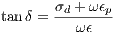 | (2) |
The second method is to use a complex permittivity:
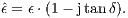 | (3) |
If we replace every relative permittivity in E_R with it’s respective complex relative permittivity, we can obtain the conductance matrix as the imaginary part of the complex capacitance matrix, without assuming a homogeneous medium. If the relative permittivity is all real, the algorithm will return an all-zero conductance matrix.
There are several ways to specify the MTL setup. The first method is basically a convenient way to specify simple setups, as it allows for circular elements only, but is therefore easy to use. The second method is more flexible, it allows for arbitrarily shaped elements, however it is more complicated to use. To determine the per unit length parameters of capacitance, inductance and conductance, the cross-section of the MTL setup needs to be given, plus the relative permittivity in the problem region. All input lengths are assumed to be in metres.
This is the first input method, that allows only for circular elements. The method is called “genMatCirc.m”, as it generates the matrices needed in the main program for circular conductors. In the file itself two boolean variables can be set: PLOTINPUT controls whether the setup as it will be returned should be plotted, and DEBUG can be used to enable some console outputs. If no screen can be found, plotting will be disabled regardless of PLOTINPUT.
There are two input variables to this method:
The variables needed in the struct or file desc are the following:
With this file, conductors and dielectrics of arbitrary shape and size are supported. In contrast to the first input method, the shape elements of the MTL setup are not specified using variables, but an image. It is therefore possible to paint the MTL setup. The actual input to this file consists of an image of the setup, and an explanatory description file that assigns properties like the relative electrical permittivity to the painted shapes in the image. The mapping is done using the colours, therefore every element of the MTL setup needs to be painted in a different colour, and that colour needs to be specified when giving further properties of that element. Again, there are two inputs to the method:
The .mat-file must contain the following variables:
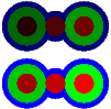
Example: You want to specify two ribbon cables with a total of three conductors each, the outer two conductors are each surrounded by a sheath, and both of the three wires are surrounded by an outer sheath. The two ribbon cables are stacked on top of each other vertically. The setup is depicted in figure 1.
The conductors are painted in different shades of red, namely (from top left to bottom right): (38,0,0), (79,0,0), (117,0,0), (161,0,0), (196,0,0), (255,0,0). The four inner sheaths are painted in green (again from top left to bottom right): (0,51,0), (0,119,0), (0,187,0), (0,255,0). The outer sheaths are painted in blue, the upper one in dark blue (0,0,119), and the lower one in bright blue (0,0,255). All values are RGB-values, where 0 is the lowest and 255 is the highest value. Let us furthermore assume that the sheaths that surround the outer two conductors of the upper ribbon cable have a relative electrical permittivity of ϵr = 2.1, the sheaths surrounding the outer two conductors of the lower ribbon cable have ϵr = 2.5, the upper outer sheath has ϵr = 3, and the lower one ϵr = 3.5. The loss tangent of the circular sheaths around the conductors is tanδ = 0.02, and the loss tangent of the outer sheaths is tanδ = 0.06. The input for genMat.m would then be:
If the above methods are unsuitable, there is always the possibility to create the necessary matrices either by hand or to create a method that computes them. The method needs to provide the following return variables:
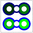
As illustration, we depicted the contents of cIm in figure 2. Notice that the dashed lines are not part of the matrices, but are for illustration purposes only and enclose the problem region. The black areas denote a “1” in the matrix, and the white areas represent a “0”.
A representation of the E_R-matrix is depicted in figure 3.
The different colours should represent the different values of ϵr, every colour is replaced with the relative electrical permittivity of the dielectric the colour represents. All pixels that are dark blue for example would be assigned the value 3. The white pixels represent ϵr = 1. Again, the dashed rectangle represents the problem region.
There are some constants that can be used to change some behaviour of the main module mtlPUL.m:
The algorithm will return the capacitance matrix C, the inductance matrix L, and the conductance matrix G for ω = 1. Notice however that the conductance matrix will be all zeros if the relative permittivity matrix E_R is all real.
Unfortunately, the algorithm we use does not converge if the problem region is too big (or the resolution is too high). It seems like the algorithm will diverge if the number of nodes in the problem region is somewhere above 30000, but it seems to depend on the shape of the region, too. On the other hand, a conductor must be represented by at least 4 nodes for the charge on the conductor to be determined properly. Therefore, there are two errors that mtlPUL.m might throw: mtlPUL:condTooSmall will be raised if one of the conductors is too small, and mtlPUL:divergence will be raised if the algorithm would diverge. If the latter is raised, it is useful to reduce the nodesPerUnit-variable, thereby reducing the number of nodes. If the first error is raised, the number of nodes must be increased. If you want to automatically compute some per unit length parameters, it is advisable to implement a little script that will catch above errors, adjust nodesPerUnit accordingly, and try again. However, if there are too many conductors in the problem region, it may occur that the problem never converges (under the condition that the conductors are represented by the necessary amount of nodes).