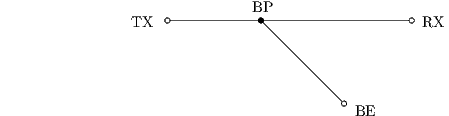
Figure 1: Cable setup
The following files should be in the MTLTF directory:
Furthermore, all files contained in the common directory are needed:
It is assumed that the common directory is in the same directory as the MTLTF directory.
Consider the following setup depicted in figure 1: Transmitter (TX) and receiver (RX) are connected by a cable. A branch cable is connected at a branch point (BP). The destination of the branch cable is called BE. We denote TX, RX, BP and BE nodes, and following the tree-terminology, we define the section between two nodes as an edge. We can identify three edges in the setup: edge one from TX to BP, edge two from BP to RX and edge three from BP to BE. The number of wires in one edge and the wires properties always remain constant (Therefore, one edge can be described by one set of PUL parameters).
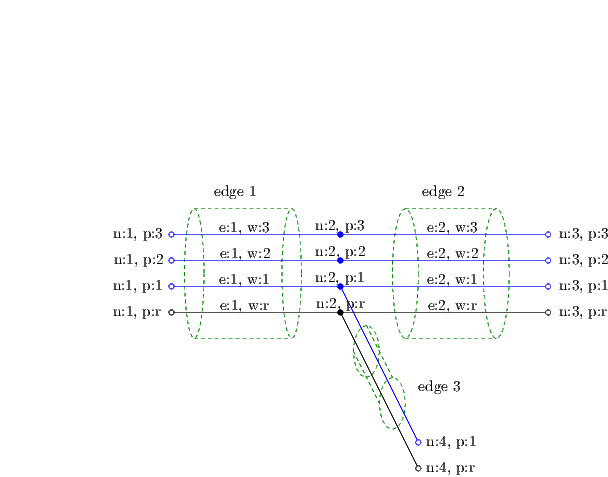
Figure 2 shows the wires inside the cables. The wires in the figure are labelled e:x, w:y, where x is the number of the edge, and y is the number of the wire in that edge. The entities where the wires can end are labelled n:x, p:y, where x is the number of the node (which is an endpoint to an edge), and y is the number of the port. A port is a entity at a node of the tree. A node may have unlimited ports. One wire connects to exactly one port at a given node (therefore, one wire connects to a total of two ports: one port at the wire’s source, and one port at the wire’s destination). Several wires may connect to the same port and wires that connect to the same port are assumed to be electrically connected at that node.
In order to describe the setup depicted above in MATLAB, we first define the set of nodes as a cell array of strings:
Then we define the edges between the nodes as a struct array with source (src), destination (dst), length (len), number of wires (numWires) and the source and destination connection arrays (srcConn and dstConn) of each edge. The connection arrays srcConn and dstConn describe how the single wires of the edges are connected at the branch point (and anywhere else in more complicated setups). A connection array is defined as follows: y = srcConn(x) means that wire number x of the edge is connected to port y at the edge’s source node.
Please be aware: Each edge needs to contain exactly one reference wire. Furthermore it is assumed that all reference wires are always connected. In the above case, we assume that wire ”r” is the reference wire. The reference wire is not accounted for in the connection arrays! We do this as the per unit length parameters used to describe the edge’s electrical properties are always with respect to a reference wire.
The “edges”-struct-array could look like this for the setup depicted above:
The srcConn array for edge one, and the dstConn arrays for edge two and three are only important when we define the load admittance matrices at those points, as they must match what we define here. (i.e, if we use 3 = conn(1), then the load admittance matrix must contain the load connected to wire one as the third entry).
Notice how the actual number of the port at the node in the middle is irrelevant, as long as all wires that are connected to it have the same number. In this case we labeled the ports from bottom to top 1, 2, and 3. (the port where the reference wires connect is not accounted for).
The now defined variables nodes, and edges, define the structure of the MTL network.
The next thing to do is to define the loads at the nodes: We use a cell array of matrices, YL, to define the loads. Every load admittance matrix is defined so that I = YL ⋅V holds, where I is the current array, and V is the voltage array. Therefore, if we have a load between one wire and ground, the entry on the main diagonal corresponding to the wire in the load admittance needs to be set to that value. If however, we have a load between two non-ground wires (say, wire two and four), we want the following to hold true:
 | (1) |
We can incorporate this load admittance into the matrix by setting YL(4,2) = -y, YL(4,4) = y, YL(2,4) = -y, and YL(2,2) = y. In our case we assume all loads are either 50Ω, or open and are between each conductor and ground. Therefore the YL cell array could read:
Where nFreq is the number of frequencies. Notice how we said there would be no load at the transmitter. This is because we handle the input load admittance with a separate matrix:
The input load admittance matrix has only two entries, as it defines the input loads that are connected to all wires that are not part of the communication link. If we had a cable with n wires, the input load admittance matrix would therefore be of dimension (n - 2) × (n - 2) × (nFreq).
For more information on how the load admittances are defined, please refer to the thesis, or to Tonello’s Paper [1].
Now we need to define the properties of the edges. The edges’ properties are described using the per unit length parameter matrices R, C, L and G.
Now we need to assign the per unit length parameters to the edges. We use the cell array PUL to do this:
As the example shows, we may either specify the per unit length parameter matrices as structs containing R, C, L and G matrices, or we may specify a function handle that will compute the per unit length parameters. The interface for the functions is as follows: [R, C, L, G] = fun(freq), where freq is a scalar denoting the frequency in Hz at which to compute the per unit length parameter.
PUL{x} therefore holds the per unit length parameter matrices (or a function pointer to a function that computes those) for the edge between edges(x).src and edges(x).dst.
We provide several functions that compute approximations of the per unit length parameters for some typical cables:
Furthermore, we provided precomputed per unit length parameter matrices for four conductors flat, and four symmetrically aligned conductors.
We define which node is transmitter and which is receiver, and which wire is used for transmission at the transmitter:
and compute the transfer function between the transmitters first wire and all wires of the receiver:
The MTLPULTF function internally computes the MIMO transfer function satisfying the following equation:
 | (2) |
where VRX is the voltage vector at node RX (node 3 in figure 2), and VTX the one at node TX (node 1 in figure 2) . The algorithm to compute the MIMO transfer function is an adaptation from Tonello’s [1] voltage ratio approach to networks including edges with nonequal number of wires.
Using the MIMO transfer function and the input admittance, the SIMO transfer function that satisfies
 | (3) |
where VTX(i) denotes the i-th entry in VTX, is then computed in singleLineTF.
HSIMO then is a (n) × (nFreq) matrix, where n is the number of wires minus one at the receiver (in our case three), and nFreq is the number of frequency points. Note that HSIMO is not in decibel, so we could compute the insertion loss in wire one in figure 2 as follows:
[1] Fabio Versolatto, Andrea M. Tonello, An MTL Theory Approach for the Simulation of MIMO Power-Line Comunication Channels, IEEE Transactions on power delivery, Vol. 26, No. 3, July 2011
[2] S. Tsuzuki, T. Takamatsu, H. Nishio, Y. Yamada, An estimation method of the transfer function of indoor power-line channels for Japanese houses, Proc. Int. Symp. Power-Line Commun., Athens, Greece, 2002, pp. 55–59