1 Contents of the package

The following files or directories should be in the HarnessTF-directory:

input

Contains input files

pulData

Contains computed PUL parameters

tmp

Contains temporary files

assignWires.m

assigns wires to tubes, based on the tree-structure of the tubes

genRndCondPos.m

generates positions for conductors on a random basis

MTLHarnessTF.m

Computes the multiple input, multiple output (MIMO) transfer function (TF), given a set of cables and a tube tree

polarRand.m

generates equally distributed random positions in a circle

script_simpleHarness.m

example script demonstrating the use of MTLHarnessTF.

script_carHarness.m

example script for a car harness

sdbmTubeHash.m

Computes a hash for a tube setup, based on the SDBM algorithm[1].

Furthermore, all files contained in the common-directory are needed:

createTree.m

Creates a tree from nodes and edges

findEdge.m

Searches for an edge connecting two nodes, given the two nodes

findPath.m

Searches for a path between two nodes through a tree

getConn.m

Gets the connection arrays for some edge

printFun.m

Helper function that will print pretty graphs

PULYZ.m

Will compute the admittance and impedance matrices using the PUL parameters

tubeYZ.m

Computes PUL parameters for an edge.

reduceTree.m

Reduces a tree to a single line, “carrying back” the branches’ loads

singleLineTF.m

Computes the single input, multiple output (SIMO) from the MIMO TF

treeplotWText.m

Can be used to plot a tree, with descriptions at the nodes

wireTF.m

Computes the TF for a single cable

We will describe the simple example file, script_simpleHarness.m, in greater detail here. It should not be necessary to understand the other files.

2 Input of the harness structure

The purpose of this code is to simulate cable harnesses like they can be found in cars, where we have a set of known wires, which are somehow routed through a network of plastic tubes. We don’t know how many wires are in each and every plastic tube and we do not know how the wires are positioned relative to each other inside a plastic tube.

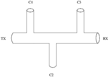
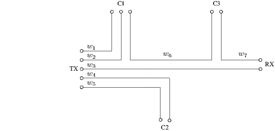
Consider figure 1:

Several wires may run in a tube. The points TX, RX, and C1, C2, C3 are supposed to be connectors. We define the points BP1, BP2, and BP3, where some wires of the tube continue into a different tube than the others.

Figure 2 shows the single cables in the tubes.

From now on we will denote the points we labeled in the above picture as nodes, and the lines between them as edges.

By comparing the first and the second picture, we can determine which wires run in which edges: In the first edge from TX to BP1, there are five wires, w₁ to w₅. In the second edge from BP1 to BP2, there are four wires: w₃, w₄, w₅, and w₆. In the third edge from BP2 to BP3, there are only two wires: w₃, and w₆. In the fourth edge from BP3 to RX again are only two wires, w₃, and w₇. In the fifth edge from BP1 to C1 are three wires, w₁, w₂, and w₆. In the sixth edge from BP2 to C2 are two wires, w₄, and w₅. In the seventh edge from BP3 to C3 are two wires, w₆, and w₇.

We don’t need to do this assignment, as the algorithm can determine it by itself given the edges and wires.

To do so using the provided algorithms, we first need to define all nodes of this graph as a cell array of strings:

and the edges that connect the nodes as a struct array defining each edges source (src), destination (dst), and length (len):

3 Definition of loads

Firstly, we define a port as an abstract concept at a node: A node may have an arbitrary number of ports, and wires may be connected to ports. All wires that connect to the same port are assumed to be electrically connected. If the node represents a connector, then the pins at the connector would be the equivalent to the ports of the node.

There are several ways to define the loads:

scalar

If only one scalar is set as load, this scalar value will be assumed to be the admittance between any wire and ground, at every node.

vector

If a vector is given, it must have one element per node. Each node will then be assigned its scalar value, which will be the admittance between any wire and ground at that node.

cell array

Must have one element per node. Each element may be:

function pointer

will be called with the number of ports at that node and the frequencies as arguments

scalar

the admittance between any wire and ground at that node will be set to this value

vector

Must have one entry per port at that node. Assumed to contain the admittance between each wire and ground.

matrix

Assumed to be the admittance matrix of that node. Must have (np)×(np)×(nFreq), where np is the number of ports at that node, and nFreq is the number of frequencies.

We use a cell array to define the load admittance matrices:

We define the input admittance matrix as

4 Input of wires in harness

The next step is to define the wires:

Where

src

Name of the node where the wire originates

dst

Name of the destination node of the wire

srcPort

Name of the port at the node where the wire originates

dstPort

Name of the port at the destination of the wire

id

unique ID for the wire

condRad

radius of the conductor

sigma

conductivity of the conductor

dielThickness

thickness of the dielectric around the conductor

e_r

relative permittivity of the dielectric around the conductor

sigma_d

conductivity of the dielectric around the conductor

gnd

true if the wire should be the reference wire.

Note that per tube only one reference wire is allowed, and no ground plane may be specified if there are reference wires.

5 Input of ground plane

If desired, a ground plane can be specified:

Where

gndSigma

conductivity of the ground plane

gndDist

distance between cable bundle and ground plane

gndHeight

height of the ground plane

gndWidth

width of the ground plane

Note: As the algorithm to compute the PUL parameters does not converge for very large areas, it is advisable to only simulate a part of the ground plane (for example that is only a little bit larger than the cable bundle. Of course this will introduce errors, but it seems like the errors introduced are rather small.

6 output

We define the transmitting node, the receiving node and the wire at which we transmit:

We can now determine the SIMO TF from any wire of the transmitter to all wires at the receiver:

The function will execute the following steps:

• create a tree from the nodes and edges variables
• determine which wires run through which tubes, and generate descriptions for each tube (how many wires run through each tube, which wires, ...)
• generate random positions for the conductors in each tube. The way the program is configured now, it will try to fit the conductors in a circular region as small as possible
• compute a hash for a tube: if we re-run the program, we don’t want to re-compute the per unit length parameter for known tubes, as this is time-consuming. The hash does not contain the position of the wires
• compute the per unit length parameter matrices for each tube, and save them using the hash as file name
• reduce the tree to a backbone, which is the shortest path from receiver to transmitter
• compute the transfer function for the backbone

References